Ever since Dynamic Arrays debuted in Microsoft 365, getting a unique list of values is easy using the =UNIQUE(A2:A999) formula. To get a count of the unique values, you would use =COUNTA(UNIQUE(A2:A999)). But these formulas count all the values in A2:A999, even those hidden by a filter.
EXCLUDING HIDDEN ROWS
Of the more than 400 functions in Excel, only two are able to optionally exclude hidden rows: SUBTOTAL and AGGREGATE. The solution to counting the number of unique customers in the visible rows involves adding a helper column to identify if each row is currently visible.
The SUBTOTAL function includes an unexpected feature when it’s used in the last row of a filtered data set. Because the AutoSum command uses SUBTOTAL to total the visible rows in a filtered data set, Excel will never hide the last row in a filtered data set if it contains a SUBTOTAL formula. This “feature” potentially breaks your ability to filter, so SUBTOTAL won’t work to solve this problem.
The AGGREGATE function was introduced in 2010 as an improvement to the SUBTOTAL function. It offers 19 calculation options, such as SUM, COUNTA, MEDIAN, LARGE, SMALL, PERCENTILE, and QUARTILE. To solve this problem, you will be using a 3 to count text entries as the first argument of the function.
The second argument allows you to specify what types of values should be excluded. There are eight options for this argument (values of 0 to 7). For example, using 0 tells the function to ignore cells with SUBTOTAL and AGGREGATE functions; a 3 ignores hidden rows as well as cells with error values or SUBTOTAL and AGGREGATE functions; a 4 ignores nothing; and a 6 ignores cells with error values. We’ll use a 5, which excludes only hidden rows.
COUNTING UNIQUE VISIBLE VALUES
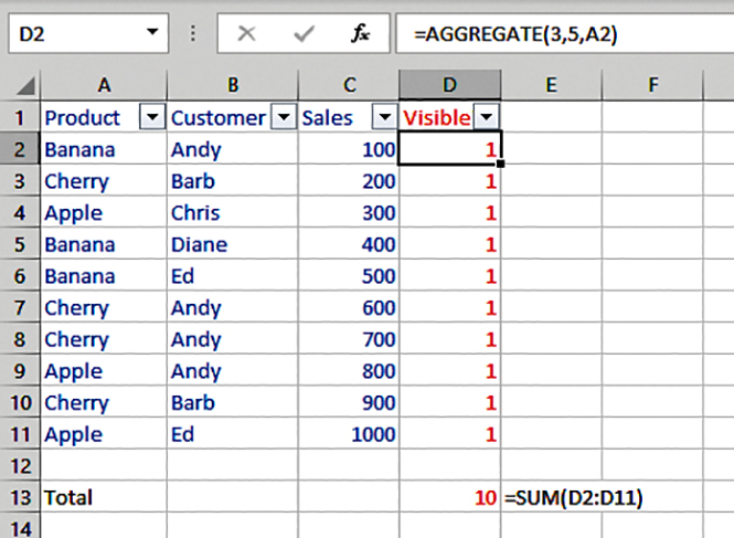
Figure 1 contains a small data set in cells A1:C11. Add a helper column to the right of the data with a heading of “Visible?” The formula in D2 is =AGGREGATE(3,5,A2). The 3 in this formula says to use the COUNTA function to count cells that contain text or numbers. The 5 says to ignore hidden rows. The A2 reference says to count how many cells there are in column A of this row. When a row is visible, column D will contain a 1. You can see the SUM function in D13 returns a total of 10.
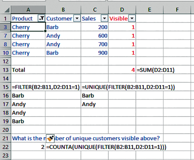
When you apply a filter to the data, the AGGREGATE function on the hidden rows will return a 0 instead of a 1. While you can’t see the zeros in Figure 2, you can tell from the SUM function in D13 that the values in rows 2, 4-6, 9, and 11 must have changed to a zero.
The AGGREGATE function in the Visible? column provides a way to operate on just the visible rows in the data set. Now we can apply the solution to get the list of unique customers displayed. A temporary formula in cell A16 uses =FILTER(B2:B11,D2:D11=1) to return a list of customer names from the visible rows. This formula spills to A16:A19 and gives you the list: Barb, Andy, Andy, Barb.
In cell C16, a temporary formula of =UNIQUE(FILTER(B2:B11,D2:D11=1)) returns one occurrence of each customer: Barb, Andy.
Finally, the formula in A22 counts the number of text entries returned by the UNIQUE function: =COUNTA(UNIQUE(FILTER(A2:A11,D2:D11=1))).
SINGLE-CELL AGGREGATE
Note that it’s somewhat unusual to specify a single cell in the AGGREGATE function. Normally, the AGGREGATE function would be pointing at your entire data set. If you wanted to calculate the median value of the visible rows, you could simply use =AGGREGATE(12,5,C2:C11). In this formula, 12 indicates MEDIAN, 5 indicates to ignore the hidden rows, and C2:C11 is all of the sales figures in the data set. In this case, you wouldn’t need the helper column to identify which rows are hidden.
As Microsoft continues to add new functions to Excel, it’s more likely that you might want to use a new calculation that isn’t one of the 19 calculations supported by AGGREGATE. In these cases, you can use the single-cell AGGREGATE in the helper column to handle detecting if a row is currently visible or not.

June 2021


