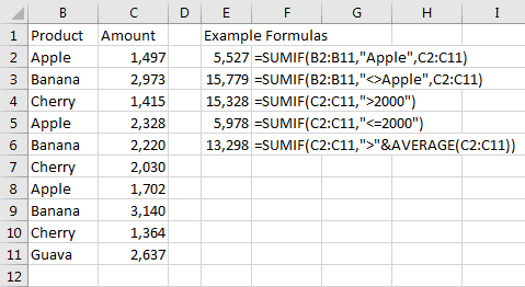
Before introducing the technique, here’s a quick review of how criteria arguments work in formulas such as COUNTIF and SUMIF. Most people are familiar with using a single value in the formulas, such as =COUNTIF(B2:B11,“Apple”). You can also expand on the single criterion using <, >, <=, >=, or <>. For example, this formula would count all of the records that are not Apple: =COUNTIF(B2:B11,“<>Apple”).
In a similar fashion, you could count all of the revenue amounts greater than $2,000 using =COUNTIF(C2:C11,“>2000”). To count all of the revenue amounts less than or equal to $2,000, use =COUNTIF(C2:C11,“<=2000”). To count all of the revenue amounts greater than average, use =COUNTIF(C2:C11,“>”&AVERAGE(C2:C11)). Similar criteria arguments can be used with SUMIF, AVERAGEIFS, COUNTIFS, SUMIFS, MAXIFS, and MINIFS.
Simply put, the Albuquerque method for filtering involves entering the criterion argument from those formulas in the first blank row below your data set and then applying the Filter by Selected Cell’s Value command.
SAVING CLICKS
Filter by Selected Cell’s Value is always three clicks away. First, you right-click on the cell containing the value to filter. In the menu that opens, choose Filter, and then Filter by Selected Cell’s Value. But if you filter often, you can get even more benefit from this technique by adding the command to the Quick Access Toolbar.
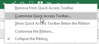
Right-click anywhere in the Ribbon and choose Customize Quick Access Toolbar.
In the dialog window that opens, go to the drop-down menu labeled “Choose commands from” and select either “Commands Not in the Ribbon” or “All Commands.” If you then scroll through the list of commands in the left list box, you won’t find Filter by Selected Cell’s Value. The old AutoFilter icon will perform the same logic, however, so select AutoFilter. Click the Add>> button in the center of the screen to add it to the Quick Access Toolbar, then click OK. Now you’re ready to try the new technique.
QUICK AND EASY FILTERING
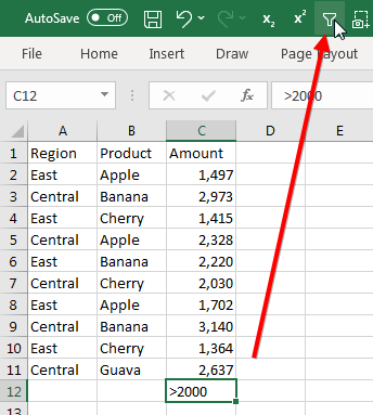
As shown in the figure below, the data set runs from A2:C11. You want to see only the rows with revenue greater than $2,000. Go to the end of the data and enter >2000 in the first blank cell below the Amount column. In this case, it’s cell C12. Note that Excel treats this as text, so there’s no need to wrap it in quotation marks.
With C12 selected, click the AutoFilter icon in the Quick Access Toolbar.
After applying the AutoFilter, only the rows with amounts greater than $2,000 are shown. What about the cell containing >2000 in C12? Since it’s text, it’s ignored by the numeric filter and that row is hidden. (You can access the row later by using Data, Filter or Data, Clear Filter to remove the filters.)
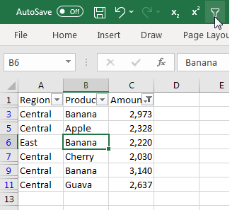
Another great trick is that you can add additional layers of filtering with the AutoFilter icon on the Quick Access Toolbar. Within the filtered data, select any cell in column B that contains “Banana,” as shown in Figure 2. When you click on the AutoFilter icon in the Quick Access Toolbar, Excel will further filter the data set to show you only sales of bananas greater than $2,000.
One caveat is that the AutoFilter icon won’t perform the Filter by Selection logic in data that has been set as a Table using the Format as Table command or Ctrl+T. If you regularly use Ctrl+T to format your tables, you can still perform the same logic with either >2000 or Banana by right-clicking the cell and choosing Filter, Filter By Selected Cell’s Value.
MORE FILTERING TECHNIQUES
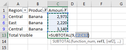
Variations of this method can provide even more filtering possibilities. The AutoSum command in Excel usually enters a SUM function for the adjacent data set. If you apply a filter to a data set first and then perform the AutoSum from the first visible empty cell below a numeric column, however, Excel will provide an ad-hoc total of the rows visible from the filtered data set. For example, after adding >2000 in cell C12 and clicking Autofilter, select cell C13 below the filtered data set and perform AutoSum. Instead of using =SUM, Excel instead will use =SUBTOTAL(9,C2:C12), giving you a total of only those cells visible.
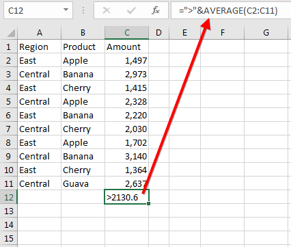
If you want to see all records that are above the column’s average, replace the >2000 in C12 with the formula =“>”&AVERAGE(C2:C11).
When you click the AutoFilter icon in the Quick Access Toolbar, Excel will filter to the rows that are above the average of column C.
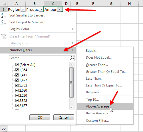
I love doing Excel seminars for IMA chapters because I always learn a few new techniques like these. While the Albuquerque technique works and saves a few clicks, I always wonder if the Excel team deliberately planned for it or if it’s just working by accident. While the Filter to Above Average technique works for static values, you can’t change the numbers and then click Reapply. Had the Excel team intended for this feature to work, I believe it would have reevaluated the AVERAGE formula. A safer alternative (though it requires extra mouse clicks) is to open the Filter drop-down menu in cell C1 and choose Number Filters, Above Average.
Bill Jelen’s new edition of Pivot Table Data Crunching Excel 2019 will be available in bookstores this month. Send questions for future articles to IMA@MrExcel.com.

February 2019


