Excel: Replacing Volatile Conditional Formatting

I was presenting at the PricewaterhouseCoopers (PwC) offices in Melbourne, Australia, for the Excel Summit South when someone in the audience had such a spreadsheet. Through a group effort, we determined that replacing the traditional conditional formatting with an old custom number format created a way to flag the same cells without causing all 600,000 cells to be volatile. The worksheet speed instantly improved.

USING VOLATILE CONDITIONAL FORMATTING

Figure 1 shows six different ways to flag cells. Any time that a value falls below 90, you want to highlight the cell.

Column A contains an icon set from the conditional formatting menu. While the flags look great, they are volatile. To have only the red flag appear on values less than 90, follow these steps:

1. Select the cells to be formatted.

2. Go to Home, Conditional Formatting, Icon Sets, 3 Flags.

3. Select Home Conditional Formatting, Manage Rules, Edit Rule.

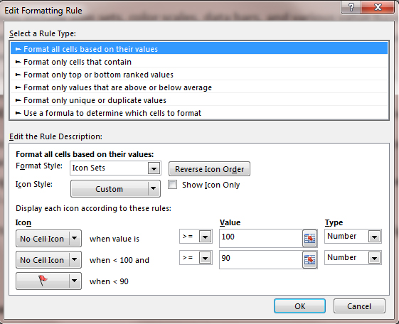
4. In the Edit Formatting Rule dialog, change the Icon to “No Cell Icon” for the first two rows. Change the Type to Number for the first two rows. Change the Value to any number larger than 90 in the first row and to 90 in the second row. (See Figure 2.)

5. Click OK to close the Edit Formatting Rule dialog, and then click OK to close the Conditional Formatting Rules Manager.

The result is a red flag appearing next to any values below 90. Because these flags use conditional formatting, they will be reevaluated during every worksheet calculation.

CUSTOM NUMBER FORMATTING

Columns B through G of Figure 1 show six possible ways (out of hundreds) to flag cells using custom number formatting. While these methods aren’t as elegant as the red flag used in column A, they allow you to flag certain values without making every cell volatile.

To apply custom number formatting, you follow these steps:

1. Select the cells to be formatted.

2. Press Ctrl+1 to open the Format Cells dialog.

3. On the Number tab, select Custom.

4. In the Type box, enter a custom number formatting code (discussed below).

5. Click OK to close the Format Cells dialog.

The custom number formatting code is usually composed of four zones that are separated by semicolons. The zones are used to specify a different format for positive, negative, zero, and text values. For example, the built-in Accounting number format uses the following code: _($* #,##0.00_);_($* (#,##0.00);_($* “-”??_);_(@_). (See Figure 3.)

Instead of automatically applying the zones to positive, negative, and zero, you can specify a condition in square brackets to be used for zones 1 and 2. The optional final zone is used to specify a number format for any cells not meeting the first two conditions.

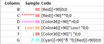
For example, column B in Figure 1 uses [red][<90]0 as the number format. In this format, [red] specifies a color, [<90] is the condition, and 0 is the number format. You could change the 0 to be any type of number format, such as $#,##0.00.

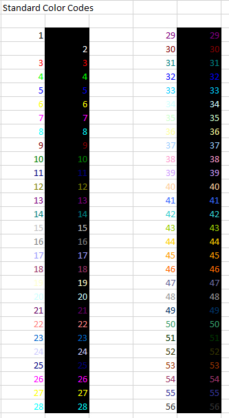
You can use any of these colors: [Black], [Blue], [Cyan], [Green], [Magenta], [Red], [White], or [Yellow]. You also can use [Color1] through [Color56], which correspond to the old Excel 2003 color palette. Figure 1 shows the pink from Color26 in column D, orange from Color46 in column E, and burgundy from Color30 in column F.

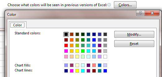
Note that you can edit the colors used for Color1 through Color56. Go to File, Options, Save, Colors, and click the Modify button to change an existing color (see Figure 4).

The standard colors in most Excel workbooks are shown in Figure 5.

OTHER NUMBER FORMAT TECHNIQUES

To simulate a check-writing machine, use ** in the number format. The first asterisk tells Excel to fill the blank space in the cell with the character that follows the asterisk. Column C in Figure 1 uses ** to fill cells less than 90 with asterisks before the number. But you can fill with any character. Column D uses *> to fill the cell with greater than (>) signs.

Any quoted text in the number format will be displayed next to the number. Column E in Figure 1 uses “Low! ”0 in the format to display the word Low! followed by a space before the number. Column F uses an upside down exclamation point. Column G uses an ó. To access these last two characters, enter =CHAR(161) or =CHAR(240), respectively, in a blank cell. Copy and paste as values. Then copy the character from the formula bar in order to paste in the custom number format box. Figure 6 shows the formatting codes used for the various columns in Figure 1.

TESTING IF VOLATILE

There’s a simple process to test if a worksheet is volatile: Save and close the workbook. Reopen the workbook and close it again without making changes. If Excel asks you to save, then you know the worksheet is volatile. When trying this test with the conditional number formatting techniques, they don’t cause Excel to ask for a save, hence they aren’t volatile.

SF SAYS

While conditions in number formats can be used to visually flag numbers, you can’t sort or filter based on colors introduced in number format codes.