A new method for inserting pictures into Excel is rolling out to Microsoft 365 customers. When you insert a picture into a cell in Excel, it’s treated as a new data type, and the picture can be used in Excel formulas.
Before this new method, pictures were inserted into a drawing layer that floats above the cells in the Excel grid. You could use the Size and Properties settings to lock a photo so it would move and/or resize it with the cells underneath the photo.
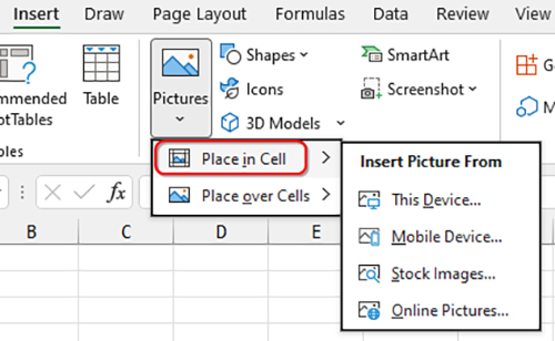
Once you have the new feature, you’ll see that Insert, Pictures leads to two choices: Place in Cell, which creates an image stored in the cell, is the new method; Place over Cells, which adds a picture on the drawing layer, is the old method (see Figure 1).
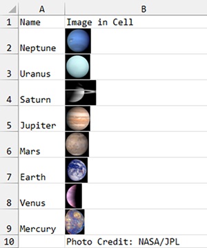
You can insert several pictures in a single command. I have a folder of some of the public domain photographs created by NASA and the NASA Jet Propulsion Laboratory. In Figure 2, with cell B2 as the active cell, I used Insert, Pictures, Place In Cell, and From This Device and selected eight planet photos. Excel embedded one image per cell, filling cells B2 through B9.
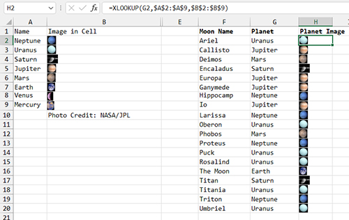
To create a lookup table, I typed the planet name to the left of each image. Note that a typical row in Excel has a Row Height of 15. This will make the images very small. For the lookup table used here, I increased the Row Height to 30. As the row becomes larger, the image will automatically resize to fill the available space. Eventually, you might need to increase the Column Width as well.
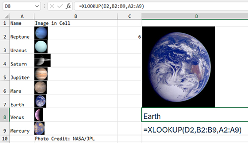
In Figure 3, I have created a larger cell by merging cells D2:D7. A formula in cell D2 will pull one of the images into D2: =INDEX(B2:B9,C2).
The images stored in a cell can be used in the XLOOKUP formula. The three required arguments in the formula are =XLOOKUP(lookup value, lookup array, return array). In Figure 3, the lookup value is the image in D2. You’re asking Excel to find that image in the lookup array stored in B2:B9 and to return the planet name from the return array in A2:A9.
The result of the formula is the name “Earth” shown in D8. Note: The ability to use the image as the lookup value was discovered by Excel MVP Leila Gharani, who posted the tip on her YouTube channel. For great Excel content, be sure to subscribe to it.
The lookup can reverse the lookup array and return array to return an image associated with a name. In Figure 4, several moons from our solar system are listed in column F. The planet that each moon orbits around is in column G. To use the lookup table in A2:A9 to get the planet image in column H, use a formula such as =XLOOKUP(G2,$A$2:$A$9,$B$2:$B$9).
Improving the Feature
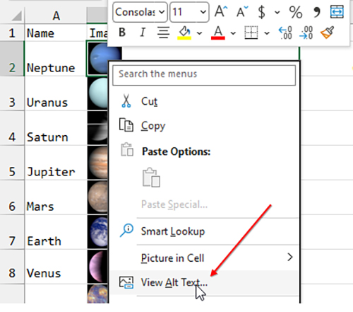
When you insert an image in a cell, the formula bar for that cell uses a generic value of “Picture.” Initially, the only way to change the name associated with a picture in a cell was to use a Visual Basic for Applications (VBA) macro to insert the image. But in July 2023, Microsoft released an improvement to Picture in Cells. As shown in Figure 5, right-click the picture in cell B2 and choose View Alt Text.
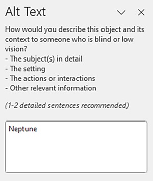
This opens the Alt Text panel on the right side of the screen. Normally, Alt Text is used to assist someone who’s using a screen reader to view your spreadsheet. The Alt Text panel suggests one to two sentences of detail for alt text. In this case, however, a simple bit of alt text of “Neptune” will suffice as shown in Figure 6. After typing “Neptune” in the Alt Text panel, click on cell B3 and add alt text of Uranus. Continue for each of the images in your table.
Note: Using the Alt Text panel is fine for a small table with two to 10 photos. If your table contains dozens or hundreds of rows, the VBA method for changing the name while inserting the image is described in this video.
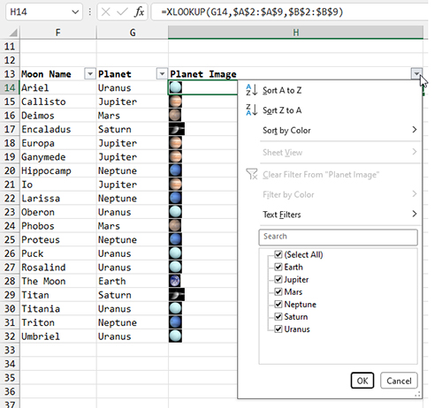
Figure 7 shows the result of adding alt text to each image in B2:B9. When the XLOOKUP formula in H14 brings the planet image into the report, it brings the Alt Text value along as well. If you use the Data, Filter command to add Filter drop-downs, the alt text is displayed in the Filter for Planet Image, allowing you to quickly filter to the moons in orbit around Jupiter.
You might use other methods for filtering, such as the AutoFilter icon in the Quick Access Toolbar, or right-clicking an image and choosing Filter, Filter by Selected Cells Value. These also work correctly after you’ve added alt text to each image in the lookup table.
Seeing a Larger Picture in a Preview Window
The new Picture in Cell feature uses the Linked Data Type feature introduced in 2018 and described in Excel: New Geography Data Type in the December 2018 issue of Strategic Finance. If you select a cell that contains an image and press Ctrl+Shift+F5, Excel will temporarily display a larger version of the image to the right of the cell as shown in Figure 8.
In Linked Data Types, the Ctrl+Shift+F5 shortcut displayed what Microsoft calls a Data Card. In the new Picture in Cells feature, the window is called a Preview. You can right-click the cell, choose Picture In Cell, Show Preview to display the card.
File Size Considerations
The Excel team used a clever method to reduce file size. When an image is initially inserted into a cell in the lookup table, the image is embedded into the Excel workbook and the size of the workbook grows. But then, if you use a formula to pull the image from the lookup table and repeat the image 100 times, the file size barely increases. For example, the image of Jupiter is 452,816KB on disk. Adding Jupiter to the workbook increased the file size by 438,475KB. But then repeating Jupiter 100 times using an INDEX function added only 1,840KB.
Embedding images inside of cells as if they were another type of data is a great improvement for Excel. There will be many applications where you can add an image of a person or a product to a dashboard report and have that image change in reaction to slicers or other inputs. If you’re eager to try out this feature now, ask your IT department to enroll you in the Office Insiders beta program for early access to features.

September 2023

