The Evaluate Formula icon found on the Formulas tab is one of the most comprehensive tools for formula debugging.
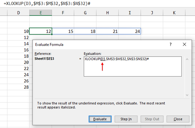
Select a cell that contains a formula. Click the Evaluate Formula icon, and Excel displays the formula in the Evaluate Formula dialog. One part of the formula will be underlined. This indicates the portion of the formula that will be calculated next.
At the bottom of the dialog are four buttons: Evaluate, Step In, Step Out, and Close. If you click Evaluate, the underlined portion of the formula will be calculated, with the result shown in the dialog. The next part of the formula to be calculated will be underlined.
In Figure 1, the first part of the formula to be evaluated is the reference to cell D3. Instead of clicking Evaluate, you could click Step In. A second, nested box appears in the dialog with the formula in D3. You can then choose to evaluate D3 one step at a time or step to any portion of the formula in D3.
The Step Out button is used to close the second formula and return to the formula shown at the top of the dialog.
TEMORARILY CALCULATE ONE PORTION
Often, you’ll be interested in just one portion of a formula. If you click into the formula bar and select that portion of the formula, you can cause Excel to calculate that portion by pressing the F9 key. Excel will replace that portion of the formula with the answer from that portion of the formula.
Once you have pressed F9 inside of the formula, you have three ways to proceed:
- Press the Esc key. Excel will clear any formula changes up to that point and exit formula editing. This can be a problem if you were building a long formula and pressed F9 on one part of the formula.
- Press Ctrl+Z to Undo. The formula will stay in editing mode, but the solution revealed by pressing F9 will return to the original part of the formula.
- Press Enter. This ruins your formula, hard-coding the subresult into the formula. I will admit that I have done this way too many times over the years.
A NEW TOOLTIP
Recently, a new change rolled out to Microsoft 365 subscribers that will be a benefit to those who frequently use the F9 key within a formula. Select any part of a formula in either the formula bar or in the in-cell editor and then hover for a moment. Excel will reveal a tooltip with the result of that part of the formula.
This is the same result that you would see if you pressed F9, but without actually inserting the calculation into the formula. In Figure 2, the tooltip with the numbers 1 to 30 show the lookup_array argument of the XLOOKUP function.
The best part: Unlike using F9, the tooltip isn’t changing your formula. You can now hover, examine the tooltip, and leave the formula intact. The feature will be rolling out slowly to the monthly and semiannual channels, so watch for it to appear in your Microsoft 365.
You might notice it when you use the Alt+= shortcut to create an AutoSum. Excel frequently proposes a range to sum and selects those characters in the formula so you can easily change the sum range. Because Excel has selected the sum range argument inside of the SUM function, the tooltip will appear with the numbers being summed.
BONUS XLOOKUP TIP
I want to share a great Excel formula tip that Financial Modeling World Cup champion Diarmuid Early passed along in a comment to one of my YouTube videos.
The XLOOKUP function used in this month’s example has a hash (#) character at the end of the function. The hash character tells Excel that you want to return all of the results of a dynamic array. In this case, the lookup table has a series of horizontal dynamic arrays in column N. Each array contains a different number of cells.
If you used =XLOOKUP(D3:M3:M32, N3:N32), Excel would return just the first cell of the array from column N. By adding the hash to the end of the formula, Excel returns the entire array that starts in column N, =XLOOKUP (D3:M3:M32,N3:N32)#.
Thanks to Diarmuid Early for passing this along. Watch Diarmuid this December 9, 2023, as the Financial Modeling World Cup returns to the ESPN family of networks.

April 2023


