A NEW OPTION
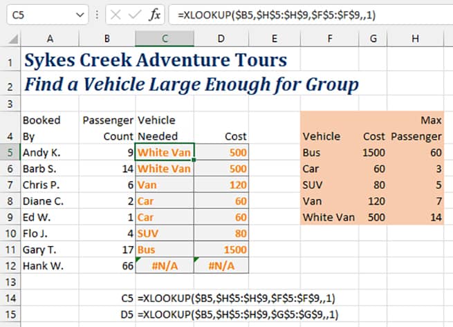
Consider the adventure tour company shown below. As it takes a reservation, it finds out the name of the person and the number of people in the party. It will need to find the correct vehicle from the lookup table shown in F4:H9. The matching technique is that you need a vehicle that can accommodate the number of passengers. If there are 1, 2, or 3 passengers, they can fit in a car. For 4 or 5 passengers, you need to reserve the SUV. Notice that the lookup table is arranged alphabetically by vehicle name instead of sorting by the passenger count.
The lookup for Barb’s group in row 6 is easy. Her party has 14 people, and the white van in row 9 of the lookup table seats 14 people. This is an exact match and something that was possible with VLOOKUP or MATCH.
The situation is more complicated with Andy’s party of 9 in row 5. There are no vehicles in the lookup table that seat exactly 9. The old VLOOKUP had an option that could find the value just less than 9, but a van that seats 7 isn’t going to work for this group.
The old MATCH function had an option to look for the next larger item, but it only worked if the lookup table was sorted in descending order by the numeric column.
VLOOKUP pros will recognize another problem: You’re looking for the passenger count in column H and need to return the vehicle and cost from columns that are found to the left of the lookup column. VLOOKUP was built on the assumption that return value was always to the right of the lookup value.
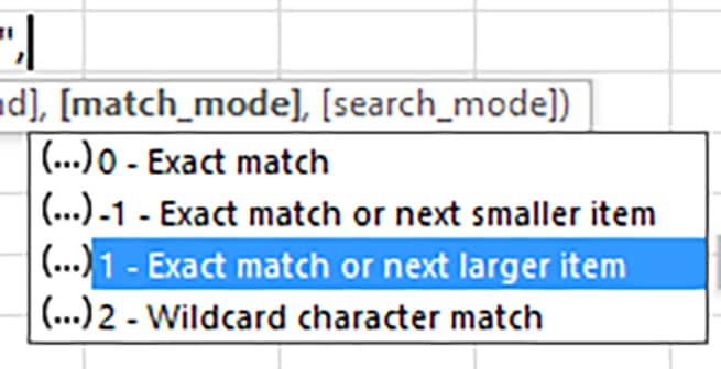
XLOOKUP is able to find the exact match or next larger item by using a match mode of positive 1, as shown here.
A CAUTION FOR MATCH USERS
For people who have used the MATCH function to find values equal or greater than the lookup value, you should carefully note the difference with the XLOOKUP match mode. In the legacy MATCH function, a positive 1 would return a value less than, and a negative 1 would return a value greater than.
Today, those directions seem backward. Why would you specify a negative number if you want to return a value larger than the lookup value? We don’t need to get into the arcane history of why they’re backward. The upside is that, with the new XLOOKUP function, Joe McDaid on the Excel team figured he could correct the meaning of positive 1 and negative 1 for the function’s match mode. As shown in Figure 2, a 0 means exact match, -1 means next smaller, and 1 means next larger. I wholeheartedly agree with this correction.
MOVING FROM VLOOKUP TO XLOOKUP
For those of you who are more used to VLOOKUP, there are a couple of simple changes to switch from VLOOKUP to XLOOKUP. Both functions start the same by providing a lookup value in the first argument. The differences come in the second and third arguments. For VLOOKUP, you would specify a rectangular table array and then an integer column number. For XLOOKUP, the second argument is a single column used as the lookup array and then a single column used as the return array.
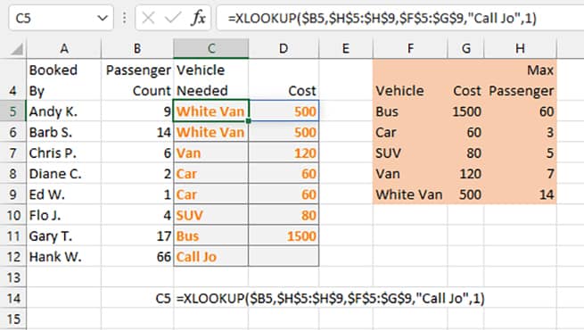
In the formulas shown in Figure 1, I skipped the optional fourth argument where you can specify what to return if something isn’t found. I actually wanted the #N/A errors shown in C12 and D12 to alert someone that there aren’t any vehicles to accommodate a tour with 66 passengers. You might prefer to return “Call Jo” instead of the N/A error. In that case, the fourth argument could be used: =XLOOKUP($B5,$H$5: $H$9,$F$5: $F$9,"Call Jo",1).
Everything is working to return the vehicle needed. When you copy the formula from C5 to D5 in order to return the cost of that vehicle, there’s a great technique to change the formula. With VLOOKUP, you would have changed the integer column number from 1 to 2 in order to point to the cost column. With XLOOKUP, you need to change $F$5:$F$9 to $G$5:$G$9. Select the copied formula in D5, then press F2 to edit. Using the mouse, drag the edge of the purple outline that surrounds the vehicle names and drop it on the vehicle costs.
Formula pros will recognize that had the original formula used F$5:F$9 instead of $F$5:$F$9, the formula would have copied correctly and automatically pointed to the cost column.
THE “SAFER” OPTION You might be wondering why I consider XLOOKUP to be safer than VLOOKUP or INDEX/MATCH. Joe McDaid describes these old functions as “brittle.” After you build the formula, it might be working fine for you. But then a person with novice Excel skills can easily break the MATCH function by sorting the lookup table or inserting a new row in the lookup table that’s out of sequence.
For the VLOOKUP function, it can easily be broken if someone inserts a new column in the middle of the table. In this case, the integer column number would need to be edited if it’s to the right of the new column.
VERTICAL OR HORIZTONTAL Note that this example uses a lookup table arranged vertically. Fans of HLOOKUP will appreciate that the lookup table can also be arranged horizontally. In that case, you would point to a lookup array and return array that’s a single row tall instead of a single column wide.
MORE FLEXIBILITY The formulas shown above use the old paradigm of each formula looking up a single value and returning a single value. I did this so the XLOOKUP would feel familiar to those used to VLOOKUP or INDEX/MATCH.
But there are two other alternatives.
You could choose to look up a single value and return both the vehicle and cost in a single formula. The formula in C5 below returns both the white van in C5 and $500 in D5. Copy the formula from C5 and paste to C6:C12.
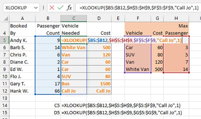
The second alternative is to look up all of the passenger counts in B5:B12 in a single formula. In this case, one formula in C5 returns all of the vehicles shown in C5:C12. Another formula in D5 returns all of the costs shown in D5:D12.
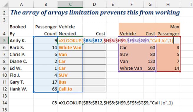
Immediately after learning both of the above examples, it’s perfectly natural to try to look up all of the passenger counts from B5:B12 and return both the vehicle needed and the cost in a single formula. This doesn’t work (yet), violating a rule that Joe McDaid describes as “the array of arrays limitation.” The return array below is expanded to attempt to return both the vehicle from F and the Cost from G. Excel only returns the vehicle from F, but it does return all of the results in F5:F12.
Looking up the next larger value, even when the lookup table isn’t sorted, is just one of the many benefits of XLOOKUP over the legacy alternatives. It’s available in Microsoft 365 and Office 2021 versions of Excel.

September 2022


