I’ve used the WEEKDAY function in combination with MOD to solve this, but the logic was always complex. The international version of the WORKDAY function provides an easier way.
HISTORY OF WORKDAY
Going back to Excel 97, Microsoft offered the WORKDAY function to deliver dates that fell on Monday through Friday. Given a starting date in cell A2, you could find the date that was three workdays later using =WORKDAY(A2,3). This was useful for making sure that nothing was ever scheduled on a weekend. An optional third argument allowed you to specify company holidays as well.
The function was useful provided your workweek was Monday through Friday. But it wasn’t useful if you lived in a country where Friday and Saturday were considered the weekend, which is why Microsoft introduced the WORKDAY.INTL function in Excel 2007. This function added an optional third argument where you could specify which days are considered weekends. The function syntax is: =WORKDAY.INTL(Start Date,Days,[Weekend],[Holidays]).
When you get to the Weekend argument while building this formula, a tooltip appears with a list of numeric codes. You would use 1 for a weekend of Saturday and Sunday; 2 would mean a weekend of Sunday and Monday. This continues up to 7 for a weekend of Friday and Saturday. The tooltip then continues with seven more options: 11 for Sunday only, 12 for Monday only, and so on.
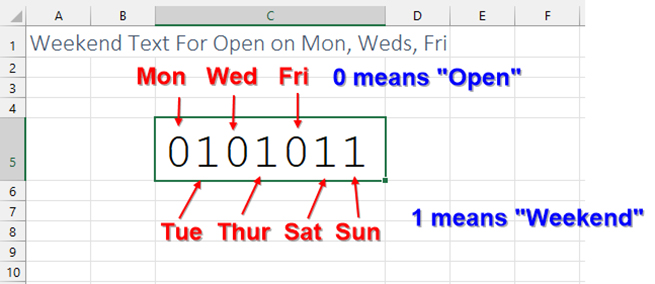
If you go beyond the tooltip and read the Excel help entry on the function, Microsoft provides an alternate way to specify which days are considered a weekend. You’re allowed to specify a seven-character text string. The first character of the text is a code for Monday. The seventh character is used for Sunday. A 1 is used to indicate a weekend. A 0 is used to indicate a workday. For example, 0000011 is a traditional workweek of Monday through Friday with Saturday and Sunday off. And 0101011 means that the workdays are only Monday, Wednesday, and Friday. A business that’s closed on Wednesday and Sunday would use 0010001.
If you want to make sure that the date calculated by the formula falls on a Friday, use 1111011 for the Weekend argument. This tells Excel to treat every day except Friday as a weekend.
COMBINING WITH EOMONTH
The EOMONTH function can be used to find the end of a particular month. It accepts a date and the number of months. To find the end of month of a date stored in cell A2, you would use =EOMONTH(A2,0). To find the end of the next month, use =EOMONTH(A2,1). To find the end of the previous month, use =EOMONTH(A2,-1).
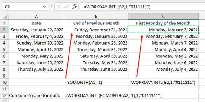
EOMONTH and WORKDAY.INTL can be used together to find things such as the first Monday of the month. Say that you have a date in cell A2. Your first step is to back that date up to the end of the previous month by using =EOMONTH(A2,-1). From there, you want to move forward to the next workday using a Weekend argument of “0111111”. Figure 1 demonstrates the EOMONTH results in column B and the WORKDAY.INTL results in column C. You could combine these two formulas into a single formula of =WORKDAY.INTL(EOMONTH(A2,-1),1,“0111111”).
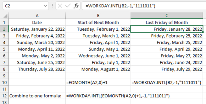
You can also combine EOMONTH and WORKDAY.INTL to find the last Friday of a month. From a date in cell A2, your first step is to find the first day of the next month. One easy way to do this is to use =EOMONTH(A2,0)+1. From there, you want to move backward to the previous workday. Specify -1 as the Days argument and “1111011” as the Weekend argument to WORKDAY.INTL. As shown in Figure 2, you could combine both formulas into: =WORKDAY.INTL(EOMONTH(A2,0)+1,-1,“1111011”).
OTHER USES OF THE WEEKEND ARGUMENT
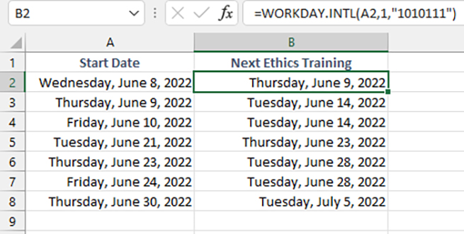
By taking advantage of the Weekend argument, WORKDAY.INTL can be adapted to many scheduling tasks. Say that all new hires need to attend an ethics training meeting, which is offered on Tuesday and Thursday. The training shouldn’t happen on the employee’s first day, but the first Tuesday or Thursday thereafter. Given a start date in cell A2, you could find the next Tuesday or Thursday using =WORKDAY.INTL(A2,1,“1010111”).
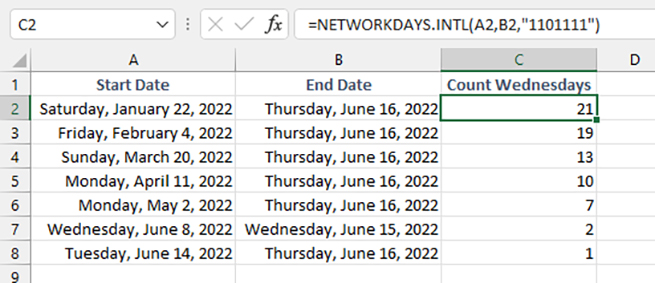
The Weekend argument is also found in Excel’s NETWORKDAYS.INTL function, which returns the numbers of workdays between two dates. For example, if you need to calculate the number of Wednesdays between dates stored in cells A2 and B2, you could use =NETWORKDAYS.INTL(A2,B2,“1101111”). Note that if the start or end date falls on a Wednesday, it will be counted.

June 2022

