The example involves data on sales by region. The spreadsheet contains columns for Product, Region, Sales Rep, and Revenue. The question involves finding out the differences by region for each product.
USING A CALCULATED ITEM
Pivot tables offer two similar-sounding features: calculated fields and calculated items. Calculated fields are used when performing calculations involving other fields in the pivot table. Calculated items are used when the calculations are within a single pivot table field. Because East and West are two items within the single Region column, you would want to create a new calculated item to do any comparisons between the two.
Create a pivot table with Product in the Rows area, Region in the Columns area, and Revenue in the Values area. This will add columns for both East and West to the report. Before starting to add a calculated item, you should choose either the East or West cell in the pivot table column headings. The selected cell tells Excel that your new calculated item belongs to the Region dimension. Had you chosen a field that contains a product name, you would be inserting a new calculated item along the product dimension.
From the PivotTable Analyze tab, open the drop-down menu for Fields, Items, & Sets. Choose Calculated Item.
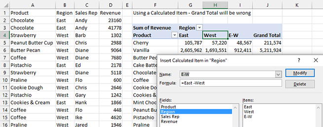
In the Insert Calculated Item dialog, give the new item a name. Since the column is relatively narrow, I went with “E-W” as the field name instead of “East minus West.”
The Formula box always starts out with a formula of = 0. You need to click in the box and backspace to remove the zero. In the Fields list box, Region is already selected. This brings up East and West in the Items list box. Double-click East to insert it into the formula. Type a minus sign. Double-click West to insert it into the formula. Your formula should now be =East - West. Click OK to add the item to the pivot table (see Figure 1).

Look closely at the Grand Total column in Figure 1. This is always a problem with calculated items. For an unknown reason, the Grand Total column treats the new calculated item as if it should be added to the other items along the dimension. While 105,787 and 57,220 should total to 163,007, the Grand Total shown in cell J5 includes the extra 48,567 from cell I5. The solution? Right-click on the Grand Total heading and choose Remove Grand Total.
The calculated item approach is easy and flexible. If you need to show East to West as a ratio, you could use the same steps to build =East/West or even =(East-West)/East.
MULTIPLE VALUE FIELDS AND SHOW VALUES AS
A different approach is to use the Value Field Settings to change the calculation in the pivot table. In this case, create a pivot table and drag the Revenue column to the Values area three times. When you have multiple fields in the Values area of a pivot table, a virtual field tile called ∑ Values appears in the PivotTable Fields pane. The tile initially appears below Region, so you need to drag the tile to appear above Region.
The three fields in the Values pane will initially be called Sum of Revenue, Sum of Revenue2, and Sum of Revenue3. Select each of those headings and click on Value Field Settings in the PivotTable Analyze tab of the ribbon.
For Sum of Revenue, simply rename the field to “Total.”
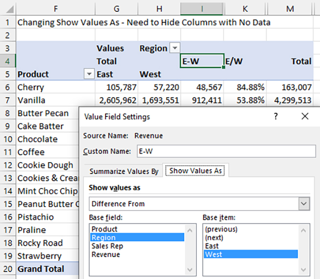
For the Sum of Revenue2, use a name of E-W. In the Value Field Settings dialog, click on the Show Values As tab. In the first drop-down below Show Values As, choose Difference From. In the Base Field list box, choose Region. For the Base Item, choose West. This will show a calculation of East minus West, as shown in Figure 2.

For the Sum of Revenue3 field, use a name of E/W. Apply the same settings as with E-W, but choose % Difference From.
The drawback to this approach is that while the Total column is correct, extra columns will appear in the pivot table. Notice in Figure 2 that columns J, L, N, and O have been hidden.
While both methods discussed here allow you to keep your calculations inside the pivot table, both have minor drawbacks and require removing or hiding some fields that don’t make sense in the final pivot table.

April 2022


