The ability to link data from two worksheets debuted as an add-in in Excel 2010. It was built into Excel 2013, but the relationship-building tools that help make it easy to do first arrived in Excel 2016.
Say that you have a large invoice register on Sheet1 with fields like “Product ID” and “Customer Number.” If the data on Sheet2 is a product database and the data on Sheet3 is a customer list, then you can easily build a pivot table from data from all three worksheets without doing a bunch of VLOOKUP formulas to get the data back onto Sheet1.
FORMAT DATA AS A TABLE
The Format as Table icon on the Home tab (or Ctrl+T) sounds like it’s made for quickly formatting a worksheet. But those words, “Format as Table,” undersell how much happens when you make a worksheet into a table. Behind the scenes, it will make a data set eligible for use in the Relationships dialog.
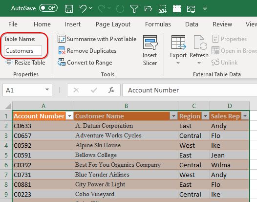
On each of the three worksheets, select the individual data set and press Ctrl+T. Excel will ask you to verify that your data has a header row. Click OK to create the table. By default, these three tables will be called Table1, Table2, and Table3. You can easily change the name of each table before you build the relationships: Select a cell in the table. A Table Design tab appears in the ribbon, and the Table Name can be edited in a box on the left side of the ribbon. For this example, call the three data sets “Data,” “Products,” and “Customers.”

DEFINE RELATIONSHIPS
If you’re using Excel 2016 or newer, you’ll see a Relationships icon in the Data Tools section of the Data tab of the ribbon.

Click the Relationships icon to open the Manage Relationships dialog. On the right side of the Manage Relationships dialog, click New… to create the first relationship.
In the Create Relationship dialog, specify the Data table has a column called ProdID. It’s related to the Products table using the column called Product.

Click New… again and define a second relationship. This one should specify that the Data table has a CustID column that’s related to the Account Number column in the Customers table.
After creating both relationships, they’ll be listed in the Manage Relationships dialog. Click Close to close this dialog.

CREATE THE PIVOT TABLE
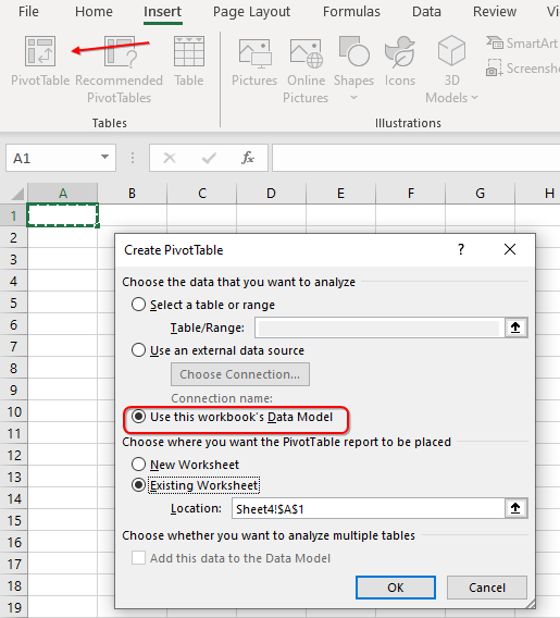
This next step is counterintuitive because most people start a pivot table by selecting the data that they want to appear in the pivot table. But for our purposes, you need to insert a blank worksheet in your workbook or simply start from a blank cell on Sheet1 and go to Insert, PivotTable.
When you start from a blank cell after defining relationships, the Create PivotTable dialog will default to “Use This Workbook’s Data Model.” This sentence always seems cryptic to me. What’s a data model? The answer is that by creating relationships, you unknowingly created a data model that lives in the workbook. The data model contains pointers to the three tables and defines the relationships between those tables.

The first thing you’ll notice in the PivotTable Fields pane is a list of table names instead of a list of field names. Each table has a greater than sign (>) to the left of the table name. Click that icon to reveal the fields available in the table.

SELECT FIELDS FROM ANY TABLE
The power of the data model happens here. You can choose Quantity from the Data table, Region from the Customer table, and Vendor from the Products table. Microsoft will join the data from the three tables much like a query in Access or SQL Server. You don’t have the overhead of thousands of VLOOKUPs.
In the pivot table shown in Figure 2, the vendor names in column A come from the Product table on Sheet2. The Regions shown in row 2 are from the Customers table on Sheet3. The quantities reported in cells B3:E8 are from the invoice register on Sheet1.
STEPS IN EXCEL 2013
The Data Model was brand new in Excel 2013, and there was no obvious way to create a relationship before you built the pivot table. In Excel 2013, you would convert all three sheets to tables. From the table on Sheet1, choose Insert, Pivot Table and choose the box for “Add This Data to the Data Model.” In the PivotTable Fields pane, change from Active to All to reveal all three tables.
As soon as you select fields from more than one table, a yellow warning box appears in the PivotTable Fields pane with a button to Create Relationships. The process feels backwards compared to the easier workflow introduced in Excel 2016, but if you’re still stuck using Excel 2013, it will work.
OTHER DATA MODEL BENEFITS
There have always been two types of pivot tables. A normal pivot table based on data from a single worksheet is a Pivot Cache pivot table. A pivot table created from external data is treated as an OLAP pivot table, and a number of pivot-table features only work with OLAP pivot tables.
When you create a relationship between tables, Excel sees your data as being an external data set. This enables features such as Include Filtered Items in Totals and Distinct Count or the ability to convert the pivot table to Cube Formulas, create subsets of rows or columns, and define new calculations with the DAX formula language.
SF SAYS
Joining worksheets in the Data Model brings the relational power of Access or SQL Server to Excel.

February 2020


