Office 365 subscribers already had the ability to pull current stock prices into Excel using the Stocks data type found on the Data tab in Excel. That feature offered the current day’s open, high, low, and current price for a stock. You could also get the 52-week high and low. But most portfolio analyses need to show the trend of stock price over time, and the original Data Type functionality wouldn’t do that.
Because the Stock Data type handles intraday prices so well, the data for the STOCKHISTORY function doesn’t change throughout the day. The data for each market is updated once a day, about three to four hours after the market closes.
USING THE FUNCTION
The new STOCKHISTORY function allows for up to 11 arguments. Only the first two are required: stock and start date.
The stock argument could be as simple as MSFT for Microsoft. By default, the stock prices returned will be from a U.S. exchange. If you want the prices from a specific exchange, use a Market Identifier Code, a colon, and then the symbol. For example, XMEX:MSFT would return prices for Microsoft on the Mexican Stock Exchange. Instead of passing the stock symbol as text, you could point to a cell that contains the ticker symbol as text or to a cell that contains a stock data type.
For the start date argument, you can pass a date in quotes or point to a cell that contains a date. Using "8/1/2020" as the argument will provide stock quotes starting with August 1, 2020. You can also use calculations such as DATE(2019,1,1) or TODAY()-30 or WORKDAY(TODAY(),-90).
For example, =STOCKHISTORY("MSFT","6/1/2020") uses only the two required arguments to provide the closing stock price for Microsoft for each weekday from June 1 through yesterday.
The following optional arguments let you fine-tune the results:
- End Date. If you don’t specify an end date, Excel defaults to TODAY().
- Interval. Specify 0 for daily, 1 for weekly, or 2 for monthly. Given that history is available for decades, it seems unusual that the ability to specify quarterly or yearly was left out.
- Headers. Specify 0 for no headers; 1 for a single row of headers; and 2 to get a title row with the instrument identifier, then a row of headers, then the stock data. Why would you want no headers? The stock prices start from the earliest date and move to the latest date. If you want to show the data with the most recent dates on the top, you’ll have to wrap the STOCKHISTORY function in a SORT function—and the SORT function isn’t expecting headers to be present.
- Property0 through Property5. This is a clever way to specify the column sequence for the stock prices. Specify 0 for date, 1 for close, 2 for open, 3 for high, 4 for low, and 5 for volume. So, for example, if you want to return the date, close, and volume, you would specify 0,1,5 as the fourth through sixth argument of the formula. Some of Excel’s built-in stock charts require columns to be in a specific sequence. For the volume-open-high-low-close chart, you need date, then open, high, low, close. That would require a sequence of 0,5,2,3,4,1 to return the columns in an order to match the chart requirements.
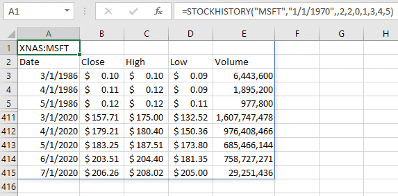
Here are some examples. Figure 1 asks for monthly MSFT date, close, high, low, volume since 1970. Note that Microsoft started publicly trading in 1986, so the first results are from March 1986. In Figure 1, I have hidden rows 6 through 410. The final result in row 415 represents July 1-3, 2020, since the figure was created on July 4, 2020.

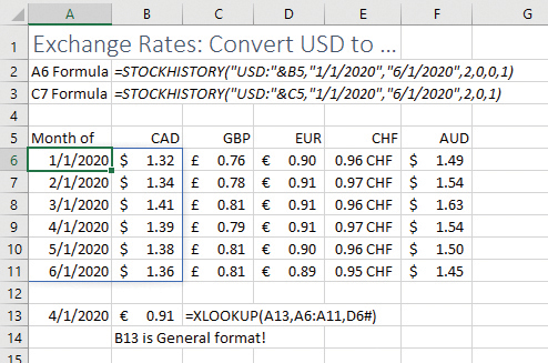
In Figure 2, a total of five formulas return year-to-date exchange rates of the U.S. dollar (USD) to the Canadian dollar (CAD), Great Britain pound, euro, Swiss franc, and Australian dollar (AUD). To get an exchange rate from USD to CAD, you can use USD-CAD or USD:CAD or even USDCAD. Note that the formula in A6 is asking for dates and closing price, and it returns column A and B. The four formulas in cells C6:F6 are asking only for closing price as they’re reusing the dates from column A.

FORMATTED NUMBER VALUES
All of the cells in Figure 2 are formatted with General format. The STOCKHISTORY function is providing a number formatting hint (called an FNV). This is new functionality in Excel. If you would change cell F5 from AUD to JPY (Japanese yen), the results in column F would automatically show up with a yen currency symbol. A formula that uses XLOOKUP, INDEX, IF, CHOOSE, or a cell reference such as =F9 will carry the number formatting to the result. Other functions such as VLOOKUP will ignore the FNV.
ERROR TYPES
There are two new error types introduced for STOCKHISTORY. First the #BUSY! error means that Excel is in the process of retrieving your results. They will appear in a few seconds. The #CONNECT! error means that you have been requesting too much data and Microsoft is throttling the results. Wait a minute or two, then use F2 and Enter to enter the formula again.
Download the Excel workbook for this month: 08Excel2020--StockHistory.
SF SAYS
Microsoft is rolling out STOCKHISTORY to Office Insiders first. It’s free to join the Insiders program.

August 2020


