An example of an approach I’ve used in the past is the Percentage Change from Previous method. This leaves an extra blank column where the nonexistent change from two years ago should be. This column needs to be hidden. When you add a new row field, the blank column moves to the right and is no longer hidden. You have to remember to manually unhide the original blank column and hide the new blank column.
Another common option is to use cells to the right of the pivot table to hold regular Excel formulas to calculate the change from the previous year. But these formulas aren’t smart enough to expand or contract as the height of the pivot table changes.
At a recent Excel seminar for an IMA® chapter, someone in the audience showed me a new method. After trying it a few times, I found it’s far more robust than the other methods and can easily adapt after new fields have been added to the row area of the pivot table.
INCLUDE A YEAR COLUMN
Start with two years of data. Assuming your data has a date column, add a formula such as =YEAR(C2) to your original data set so there’s a separate column showing just the year. Use “Year” as the heading, and copy the formula down to all rows of your data. Alternatively, you might use Power Query’s Column From Examples feature to add the column.
It’s important to add this field to the original data set and not create the field using Group Field in the Pivot Table. As we’ll see, the process involves using the Calculated Item feature, which isn’t compatible with the Year created using the Group Field command.

INSERT A CALCULATED ITEM
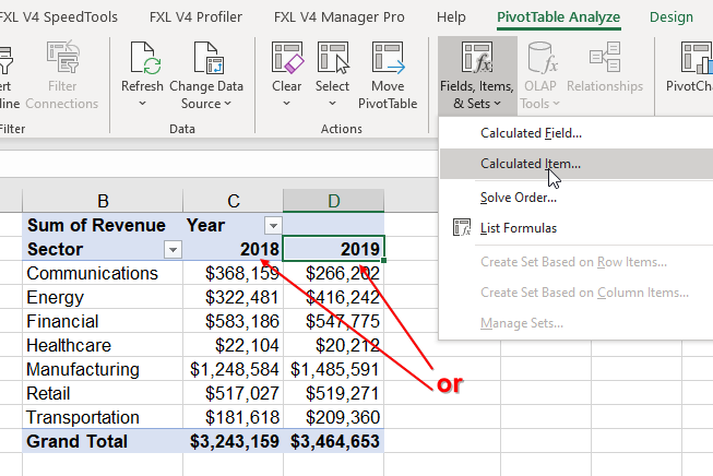
To calculate the change from 2018 to 2019, use a Calculated Item in the pivot table. It might seem subtle, but you have to select one of the column headings for 2018 or 2019 before invoking the command. Select the heading for 2018. On the PivotTable Analyze tab, open Fields, Items, and Sets. Choose Calculated Item.

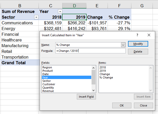
A dialog box for Insert Calculated Item in “Year” will appear. Give the new item a name, such as “Change.” The formula always starts out as =0. You need to click at the end of the formula and backspace to remove the zero from the formula. You can then double-click on the 2019 item from the right side of the dialog box to insert ‘2019’ in the formula. Type a minus sign. Double-click on ‘2018’ so the formula reads = ‘2019’ – ‘2018’.

When you click OK, a new column showing Change will appear in the pivot table.
You can use the first calculated item to calculate future calculated items. With cell C2, D2, or E2 selected, use Insert Calculated Item again. Call this field “% Change.” The formula should be = Change / ‘2018’.

A LITTLE TRICKERY
You wouldn’t think that number formats would be a part of this technique that requires trickery, but with the calculated items, every cell in C3:F10 (see Figure 2) is seen as a Revenue cell. If you right-click on cell F3 and choose Number Format, you’ll change the format for all four columns of revenue.
Instead of using the PivotTable formatting tools, simply select the Percentage Change numbers in cells F3:F10. Use the Number group on the Home tab to select a percentage with one decimal place. This step will change the number format only for the % Change column.

Once a year, you’ll also need to edit the formula for Change to reflect the changing years. Select a year heading. Open the Insert Calculated Item dialog box. Use the drop-down arrow to the right of the Name field in order to edit an existing formula. For example, you’ll need to change ‘2018’ to ‘2019’ and change ‘2019’ to ‘2020’ once we’re into 2021.
CHANGING THE FIELDS
The other methods I’ve demonstrated over the years were hoping that you would never want to change the shape of the pivot table. If you resort to calculations outside of the pivot table, those have to be extended or contracted whenever the shape of the pivot table changes.
This new method is better because the calculations continue to work even as you change fields in the Rows or Filters area of the pivot table. For example, try removing Sector from the Rows area. Add Region and Product as new Row fields. Depending on whether you’re using Tabular or Compact layout, the pivot table could grow to six columns, with more rows as well. Excel correctly adds the new rows, and the calculated items automatically work for the new data. Even the percentage formatting expands to handle the new rows. SF

SF SAYS
There are at least three methods for calculating year-over-year in a pivot table. Each method requires some trickery.

April 2020


