SORTING AND FILTERING WITH A FORMULA
By far, the functions that seem to offer the most promise are SORT, SORTBY, FILTER, and UNIQUE. Most users are accustomed to using the sort icons or the filter tool when working with data, but there are times when you might want to sort a list but the calculations keep changing or when you don’t want to leave it to the people using your worksheet to sort or filter the data properly. Being able to use a formula to do the same tasks can save time and ensure results appear as you want them to.
For example, if you had data in cells A2:C99 that you wanted to sort descending by column C, then =SORT(A2:C99,3,-1) would accomplish the task.
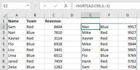
The Excel team realized that sometimes you might want to sort column A by column C and return only the values from column A. In this case, you could switch to use =SORTBY(A2:A99,C2:C99,-1).
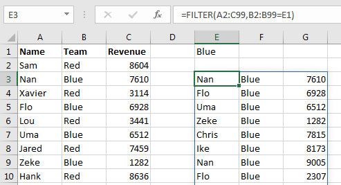
Now imagine you want to retrieve all records from A2:C99 where the team name in column B is “Red.” You can use =FILTER(A2:C99,B2:B99=“Red”). A better approach might be to enter the word “Red” in cell E1 and then refer to E1 in the formula: =FILTER(A2:C99,B2:B99=E1).
UNIQUE OR DISTINCT LISTS
Consider this simple list of six items: apple, banana, cherry, apple, banana, guava. If you wanted the unique list of products in the list, would you answer “apple, banana, cherry, guava”? If so, you’ll love the default =UNIQUE(A2:A99), which will provide exactly one occurrence of every value found in A2:A99.
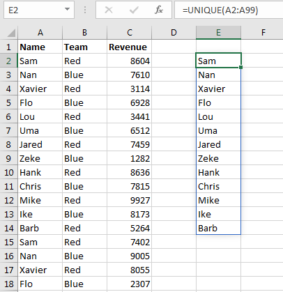
Database pros, however, might say that “apple, banana, cherry, guava” is a list of the distinct values. They would argue that only “cherry” and “guava” are unique because they’re the only products that appear exactly once. In my opinion, this isn’t the right definition, but the new function can return items that appear exactly once using =UNIQUE(A2:A99,,True).
ONE FORMULA, MULTIPLE RESULTS
With these new formulas comes a ground breaking change to the Excel calculation engine—a single formula entered in one cell is returning many rows and columns of results. The formula only exists in the top-left corner of the results. If you put the cursor on any other cell within the results, a grayed-out version of the formula appears in the formula bar. If you attempt to edit the formula from anywhere in the spill range, you’ll be directed to edit the formula in the top-left cell.
If you’re using a function such as FILTER or UNIQUE, the number of rows returned by the function can change as the input cells change. If you enter the formula in cell E2, then referring to =E2# will refer to the entire set of results.
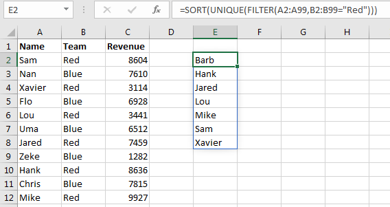
These functions can be combined, too. If E2# contains the filtered list of names from column A, you can enter =UNIQUE(E2#) in cell F2 to get a unique list of names from those results, and then add =SORT(F2#) in G2 to get a sorted unique list of names. Or, if you won’t need those intermediate results, you could do it all in a single formula: =SORT(UNIQUE(FILTER(A2:A99,B2:B99=“Red”))).
TURN OTHER FUNCTIONS INTO ARRAYS
The SEQUENCE and RANDARRAY functions seem fairly tame compared to the others. For example, =SEQUENCE(10) generates a vertical column of the numbers 1 through 10, while =SEQUENCE(10,5,4,2) generates a 10-row by 5-column sequence starting at 4 and increasing by 2. In a similar fashion, =RANDARRAY(10,5) will generate a 10-row by 5-column array of RAND() results.
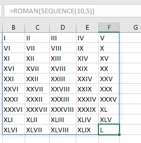
But as I began putting together examples using the new array functions, I realized that you can use SEQUENCE inside of almost any function to make that function operate as an array. For example, =ROMAN(SEQUENCE(10,5)) will generate 50 cells of Roman numerals.
And you can use =SEQUENCE(12,1,37,1) as the period argument inside of IPMT to calculate the interest for all months in the third year of a loan. SEQUENCE seems simplistic, but it unleashes power when used this way.
THIS IS GOING TO BREAK IMPLICIT INTERSECTION
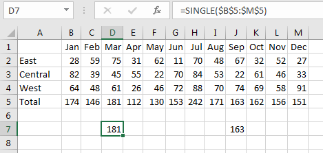
It’s rare to find people who know and love the implicit intersection function in Excel. In order for the new dynamic arrays to work, Excel had to do away with implicit intersection. If you previously relied upon =B10:M10 to return only the value from row 10 that intersects with the formula, this will no longer work. If you need this intersection to happen, you’ll have to wrap your formula in the =SINGLE(B10:M10) function.
Whenever Excel detects that you were trying to use implicit intersection, the SINGLE function will start appearing in your formulas. More often than not, people were making use of implicit intersection without realizing what was happening. If that describes you, the appearance of SINGLE in your formulas may seem confusing.
PREPARING FOR DYNAMIC ARRAYS
Note that these seven functions aren’t part of Excel 2019. You must have Office 365 to get the new functions. (In fact, the release of Dynamic Arrays on the same day that Office 2019 shipped caused Office 2019 to be obsolete the day it was released.) As of mid-October 2018, the Excel team had rolled the functions out to the Insiders channel. People on the Monthly and Semi-Annual channels will start to see these new functions in early 2019.
To get ready for these new functions, my Excel Dynamic Arrays Straight to the Point ebook will be available for IMA® members to download for free from http://bit.ly/2CV04Nz.
SF SAYS
Pressing Ctrl+Shift+Enter to create an array formula is a thing of the past with these new, simpler functions.

November 2018


