Suppose you have a list of steps that have to be accomplished to finish a task every month. The list starts in cell A3 and extends down the worksheet for a number of rows. You would like to have a checkmark appear in column B for any tasks that are complete.
Typically, checkmarks are complicated in Excel. If you use a capital P and format the cell with the Wingdings 2 font, you can get a checkmark in a cell. But unless you use checkmarks frequently, it’s difficult to remember which font and which letter is the checkmark combination. Instead, the method Jack proposed at the seminar is easier to remember and simple to create.
Jack’s system uses a green checkmark for a task that’s been completed and an empty circle for those that aren’t. When the checklist is printed, the empty circle provides a spot on which to draw a checkmark with a pen or pencil. Jack also suggests using a third symbol, such as a yellow dash, for items that should remain in the list but aren’t applicable in the current month.
At the beginning of the month, every item in the list in column A begins with a value of 0 (zero) in column B. When an item is completed, change the 0 to a 1. For any item that doesn’t need to be completed that month, enter a -1.
Here’s how you can set this up in your workbook:
- Add a 0 in column B next to each of your list items. (This won’t appear in the final result.)
- For the first task, replace the 0 in cell B2 with a 1.
- Find a task that isn’t required this month, and replace the 0 with -1.

- Select the range of 1s, 0s, and -1s in column B.
- Go to Home, Conditional Formatting, Icon Sets. Out of the 20 built-in icon sets available, 10 offer three icons and are appropriate for this task. To minimize the amount of set-up work, choose the set containing a green checkmark, yellow exclamation point, and red X.

- After choosing the icon set, you will see a mix of checkmarks, dashes, and X’s appear between each task in column A and the numbers in column B.
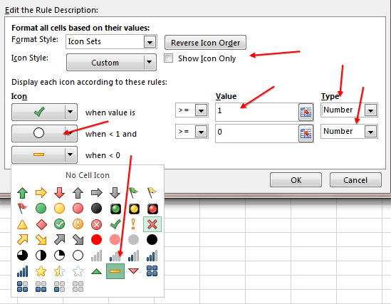
- Without selecting other cells, go to Home, Conditional Formatting, Manage Rules. Choose the Icon Set in the Conditional Formatting Rules Manager dialog and click the Edit Rule button. There are six settings to change in the Edit Formatting Rule dialog. Make sure to change them in the order indicated in steps 8-13.
- Choose the box for Show Icon Only. This will ensure that you see only the checkmarks and not the numbers.
- Open both drop-downs under Type and change Percent to Number.
- For the first box under Value, type a 1. This will indicate that any value greater than or equal to 1 will get the green checkmark.
- For the second box under Value, make sure the value is 0.
- Open the second drop-down under Icon (the yellow exclamation mark) and select an empty black circle.
- Open the third drop-down under Icon (the red X) and select a yellow dash (see Figure 1).
- Click OK to close the Editing Formatting Rule dialog. Click OK to close the Conditional Formatting Rules Manager.

Jack suggests increasing the font for column B to 18. You can also apply a strikethrough in column A to any task with a green checkmark in column B. Follow these steps:
- Select the tasks in column A.
- Go to Home, Conditional Formatting, New Rule. There are six types of rules listed. Choose the last one: “Use a formula to determine which cells to format.”
- In the Formula box, type =B3=1. This formula points to the cell to the right of the first cell in the selection. In this case, it’s cell A3. If your list starts elsewhere, adjust the formula accordingly.
- Click the Format button. On the Font tab, choose Strikethrough. Click OK on each of the three open dialog boxes.

To use the worksheet, type a 1 in column B for any item that’s complete. The empty circle will change to a green checkmark, and the words in column A will be crossed out.

You could extend this example to use four or five different symbols by choosing an icon set with that many symbols in step 5.
Download this month’s workbook to try it out for yourself: SF-2018-06-Checklist
SF SAYS
The use of Conditional Formatting avoids the need to switch to the Wingdings font for checkmarks.

June 2018


