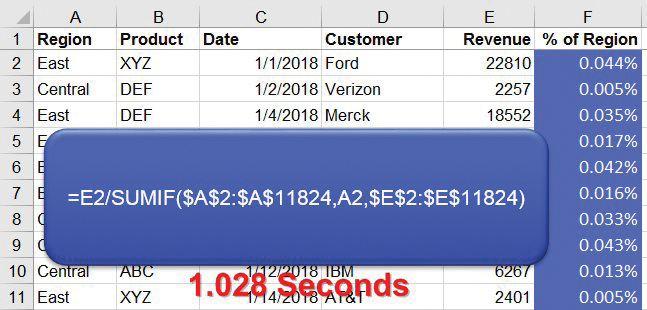
Consider the formula shown in Figure 1. Your goal is to calculate a percentage of the Region Revenue in column F. For each cell in the data, you need to divide the revenue in column E by the total revenue for that region. One way to calculate the total revenue for the East region would be a SUMIF function: =SUMIF($A$2:$A$11824,A2,$E$2:$E$11824). Divide the result from that formula into the revenue in E2, and you will have a percentage of revenue for the particular region.

The formula works. But when you copy it down into all 11,823 rows of data, the worksheet recalculation time slows down. On my desktop PC, it actually takes 1.028 seconds to calculate column F. Any worksheet that takes longer than one-third of a second to recalculate will become frustrating to anyone trying to enter data.
I’ve heard some Excel experts claim that the new SUMIFS function is faster than SUMIF. In my tests, the SUMIFS function is calculating in 1.041 seconds, slightly slower than the equivalent SUMIF.
Whether you’re using SUMIF or SUMIFS, the problem is that you’re calculating the same answer over and over and over as the divisor in the formula. In Figure 1, cells F2 and F4 are both calculating the total revenue for the East region. If the total revenue for the East is $52,353,063, then the formula in F2 will be calculating 22,810/52,353,063 and the formula in F4 will be calculating 18,552/52,353,063. The bottleneck is that Excel has to take the time to calculate the $52,353,063 divisor every time it encounters a record for the East region. Figuring out the total revenue for a region using SUMIF requires Excel to examine 23,646 cells.
A HELPER RANGE
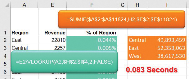
The solution is to move the bottleneck—the repeated portion of the calculation—to a set of helper cells. In Figure 2, the formulas in cells I2:I4 calculate the total revenue for each of the three regions. The formula in I2 is =SUMIF($A$2:$A$11824,H2,$E$2:$E$11824). These three calculations will take as long as the identical calculations in F2:F4 in Figure 1. The advantage is that Excel won’t have to repeat the calculations in rows 5 through 11,824.
Once you have the total revenue for each region in cells I2:I4, the formula in cell F2 can be changed to be =E2/VLOOKUP(A2,$H$2:H$H4,2,FALSE). Even though VLOOKUP usually slows calculation times, the lookup table is only three rows. The entire worksheet in Figure 2 will calculate in 0.083 seconds—12 times faster than the formula in Figure 1.
CAN THE VLOOKUP BE FASTER?
In an effort to try to make the formula in Figure 2 even faster, I tried changing the VLOOKUP to use TRUE as the fourth argument instead of FALSE. In my tests with a three-row VLOOKUP table, the recalculation times were nearly equivalent.

Here’s why it’s nearly the same. The FALSE version of VLOOKUP will always start in row 1 of the lookup table and examine each row in sequence. With a three-row table, the FALSE version of VLOOKUP will look at row 2, then row 3, then row 4. If you’re looking up Central, it looks only at row 2. If you’re looking up East, Excel will look at rows 2 and 3. If you’re looking up West, Excel will look at rows 2, 3, and then 4.
The TRUE version of VLOOKUP is smarter. It starts in the middle of the table and then will jump to the middle of the top half or bottom half of the table. In this case, it starts at row 3. If you happen to be looking up East, it can stop there. Excel then makes a decision to either move to row 2 if you’re looking up Central or row 4 if you’re looking up West. This seems brilliant: Excel will never have to examine more than two rows in the three-row lookup table.
At best, you’re saving Excel from looking at three rows in the table when it goes to find West. For Central, Excel will be looking at two rows instead of one. For East, Excel will be looking at one row instead of two. This might save you 16.7% of recalculation time. But, at this point, it’s 0.167 of 0.083 seconds, which is only around 0.01 of a second. The TRUE version of VLOOKUP also introduces risk: It can return a wrong result if a user doesn’t keep the lookup table sorted ascending.
SF SAYS
Isolate any repeated portion of a formula and move that formula fragment to helper cells.

January 2018


