DESELECT CELLS
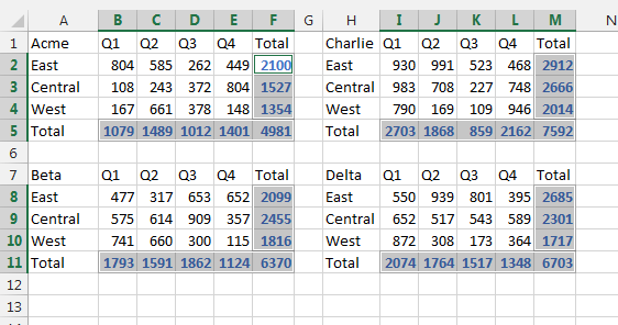
Consider Figure 1. You’ve used the mouse to select B2:E4. You then held down Ctrl and used the mouse to select B8:E10, then I2:L4. But when you did the same with cells I8:L10, you went one column too far and inadvertently selected cells M8:M10 as well. Once you released the mouse button, they were part of the selection. You had to start over again (and likely did it more slowly to make sure you didn’t slip again).

With this new feature, however, you can simply deselect the unwanted cells. Hold down the Ctrl key. With the mouse, click on M8 and drag it to M10. As you are dragging, the area becomes a lighter shade of gray. Release the mouse button, and the three cells are no longer part of the selection. It’s a tiny new feature, but you’ll be amazed at how quickly you start using it.
People who subscribe to Office 365 will have this feature in February or March 2018 (depending on your IT department’s selection on how quickly you receive new features). Those without Office 365 subscriptions will get the feature when Office 2019 is released later this year.
CELL SELECTION TIPS
There are a number of methods you can use to make selecting cells easier or more efficient.
Go To Special. You can use Go To Special to select certain types of cells, such as only those containing a formula or those with only numbers.
In Figure 1, only the total rows and columns are formulas. The rest are numbers manually typed into Excel. If you wanted to quickly select the formulas, select cells B2:M11. Then, from the Home tab, go to Find & Select, Formulas. Excel will select just the formula cells.
If you wanted to select all of the cells with numbers and not formulas, follow these steps:
- Select B2:L10.
- Choose Home, Find & Select, Go To Special.
- In the Go To Special dialog, choose Constants.
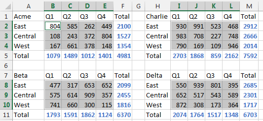
- The four checkboxes below Formulas also work for Constants. Uncheck Text, Logicals, and Errors. This leaves Constants and Numbers, as shown in Figure 2.

- Click OK. Your selection will change to only the numeric cells that aren’t formulas.
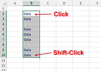
Shift Key. Another useful method is using the Shift key when selecting cells. Say that you have to select a range of cells that are a mix of empty cells and those with data. Click on the first cell. Holding the Shift button, use the mouse to click on the last cell. Excel will select everything between the two cells.
Many people don’t realize that the Shift key also can be used to select with the navigation keys. Say you are at the end of a large data set. The active cell is M659. Pressing Ctrl+Home will jump to cell A1. If you add the Shift key—Ctrl+Shift+Home—you’ll select all cells from M659 to A1.
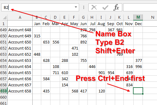
But what if you don’t want to select all the way to A1? Your data has headings in row 1 and labels in column A. So you would like to select from M659 to B2. There’s no built-in shortcut key to jump to B2, but there’s an easy way to do this:
- Press Ctrl+End to take the cursor to the last cell in your data.
- Click in the Name box (located to the left of the Formula bar).
- Type B2, but don’t press Enter.
- Hold down the Shift key while pressing Enter. Excel will select from the active cell back to B2.
Alternatively, you could use the Go To dialog (Ctrl+G) to quickly move to B2. Then press Ctrl+Shift+End to select to the last used cell in the worksheet.
Extend Selection. Press the F8 key, and “Extend Selection” will appear in the Status Bar at the bottom of Excel. When you click in any cell, Excel will select from the active cell to the newly clicked cell. The nice feature about this is that you can easily reselect a different ending cell, and Excel will always select from the active cell to the newly clicked cell.
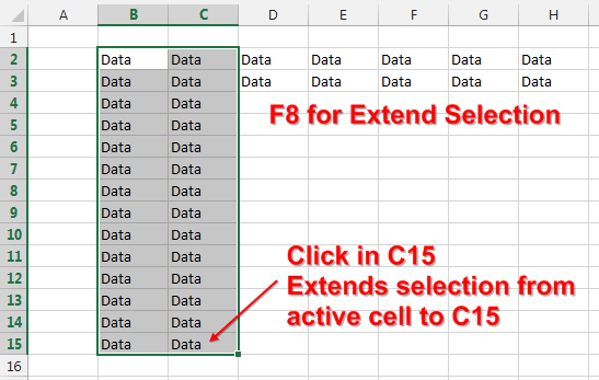
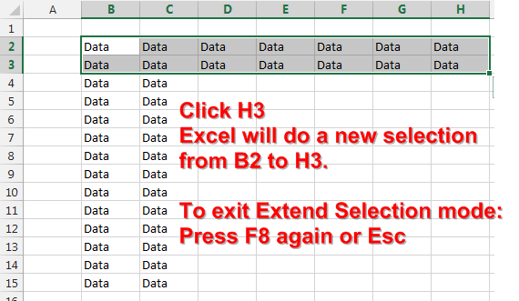
Extend Selection also works using the arrow keys. Start in cell B2. Press F8. Use the right arrow and down arrow to move the cursor around, and Excel will keep selecting additional cells until you stop pressing arrow keys.
Add to Selection. Press Shift+F8 key, and “Add to Selection” will appear in the Status Bar at the bottom of Excel. You can select additional areas using the mouse, but you don’t have to hold down the Ctrl key.
Go To. Press F5 (or Ctrl+G) to open the Go To dialog. You can type B2:M659 and press Enter to quickly select that range.
SF SAYS
Selecting multiple areas was frustrating when there was no way to deselect an errant cell. Now there’s a solution.

February 2018


