In the past, if you wanted to concatenate a list of names in column A, you couldn’t use a simple formula such as =CONCATENATE(A1:A26). Instead, you had to specify each cell individually: =CONCATENATE(A1,A2,A3,A4,A5,…A26). Unless the values stored in column A happened to have trailing spaces, you would end up with a hard-to-read result like AndyBettyCharlieDaleEddy.
TEXTJOIN offers some improvements over CONCATENATE. The syntax of TEXTJOIN is =TEXTJOIN(Delimiter, Ignore_Empty, Text1, [Text2],…).
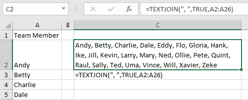
Here’s how it works:
- The first argument lets you specify a delimiter to appear between each value. For example, including “, ” would make sure that the names appear with a comma and space between them: Andy, Betty, Charlie, Dale, Eddy.
- In the second argument, you can specify that empty values should be ignored. This will prevent two consecutive delimiters from appearing. Say that you removed Charlie from cell A4. By specifying TRUE for the Ignore_Empty argument, you will get Andy, Betty, Dale instead of Andy, Betty, , Dale.
- The text arguments (Text1, Text2, etc.) can specify a range. It can be one column, like A1:A26, or multiple columns, like A1:Z26. It can even be a 3-D reference, such as ‘Jan 2018:Dec 2018’!A1:Z26.
SUPPORT FOR ARRAY FORMULAS
Array formulas are a powerful class of formulas in Excel. These formulas can perform a calculation over several cells in a range and then return the results to another function. While array formulas are powerful, they don’t work with most Excel functions. They certainly never worked with CONCATENATE.
While Excel Help doesn’t reveal it, the TEXTJOIN function does support an array as the third argument. This allows you to do some interesting calculations inside of TEXTJOIN. Say that you wanted to retrieve a list of people who RSVP’d “Yes” to an event.
You might be tempted to add a new column with =IF(B2=”Yes”,A2,””):
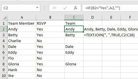
In the next figure, column A contains the names. Column B contains “Yes” or “No” for RSVP. You want to find all of the people who have a RSVP value of Yes. The array portion of the formula is IF(B2:B26=“Yes”,A2:A26,“”). In English, this formula says, “If column B says Yes, then return the name in column A; otherwise return an empty text.” The consecutive quotation marks (“”) indicate an empty value.

Using this array formula as the third argument to TEXTJOIN sends Andy, Betty, “”, Dale, Eddy, “”, Gloria to the TEXTJOIN function. If you specify TRUE for the Ignore_Empty argument, Excel will return Andy, Betty, Dale, Eddy, Gloria.
Like most array formulas, you have to use a special shortcut key. Type =TEXTJOIN(“, ”,TRUE,IF(B2:B26=“Yes”,A2:A26,“”)), but don’t press Enter. Instead, hold down Ctrl+Shift, then press Enter. Release Ctrl+Shift. This keystroke combination, called Ctrl+Shift+Enter, is required any time you enter or edit an array formula. If you do the keystroke correctly, you’ll see curly braces around the formula in the formula bar.
RETURNING ALL MATCHES FROM A VLOOKUP
The VLOOKUP function returns only the first match found in the specified lookup table. I often have people ask me if they can return all matching values.
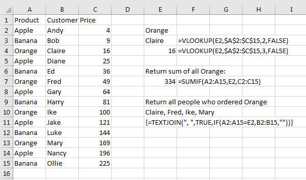
If you’re looking up numbers, you can replace the VLOOKUP with SUMIF or SUMIFS. Say that you have product in A, customer in B, revenue in C. Using =VLOOKUP(“Orange”,A2:C15,2,False) will return the first customer who purchased an orange. Using =VLOOKUP(“Orange”,A2:C15,3,False) will return the price of the first order.
Ever since Excel 97, you could sum all of the revenue from orders for oranges using =SUMIF(A2:A15,E2,C2:C15). But there wasn’t an easy way to return a list of all of the customers who had purchased oranges.
By using =TEXTJOIN(“, “,TRUE,IF(A2:A15=E2,B2:B15,”“)) followed by Ctrl+Shift+Enter, you can return a list of all of the customers who purchased an orange.
SUPPORT FOR 3-D RANGES
I was having a casual conversation with one of the Excel team project managers who wrote the specification for the TEXTJOIN function. I was thrilled when he mentioned that TEXTJOIN would support arrays. I was unsure when I would ever have a use for 3-D references, but you can specify that you want to concatenate all of the cells in all of the sheets. For example: =TEXTJOIN(“, “,True,January:December!A1:Z26) will return any value found in cells A1:Z26 of every worksheet between (and including) January and December.
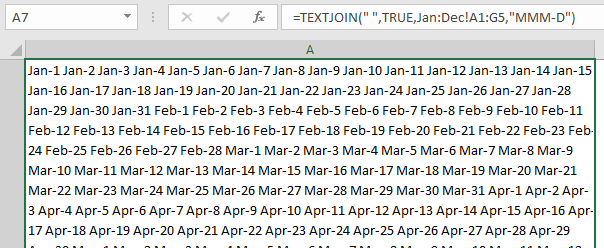
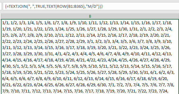
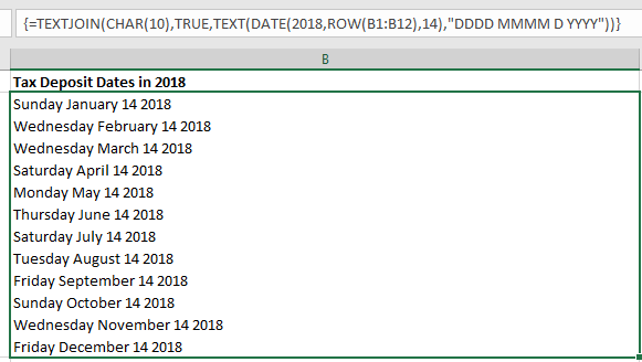
Array formula techniques also can be used inside of TEXTJOIN to generate a list of dates.
This figure uses a linefeed character, designated by CHAR(10) as the delimiter.
The TEXTJOIN function is currently only in the subscription versions of Office 365. If you own a perpetual license of Excel, you’ll have to wait until Office 2019 ships later this year for the new functionality.
SF SAYS
Along with TEXTJOIN, Office 365 subscribers can also use the new IFS, MAXIFS, MINIFS, SWITCH, and CONCAT functions.

April 2018


