Normally, you would open the Functions Argument dialog by clicking the fx icon (known as Insert Function) located on the Formulas tab of the ribbon and also to the left of the Formula Bar. Keyboard shortcut fans might know that you can start typing a formula, like =VLOOKUP(, into a cell and then press Ctrl+A to open the Functions Argument for that function.
Frequently when using Excel, though, you might need to create formulas that nest one function inside of another function—for example, like when you have to put a MATCH function inside of an INDEX or VLOOKUP function. It isn’t intuitive, but you can successfully use the Function Arguments dialog for each of the functions in the formula.
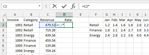
Let’s say that you need to multiply cell C2 by the result of a VLOOKUP function. The VLOOKUP is going to look for the current month’s data by using the MATCH, TODAY, and TEXT functions. Start by building the formula of =C2*.
USE THE NAME BOX
The Name Box is a dropdown menu that appears to the left of the formula bar. When you are in the middle of editing a formula, opening the Name Box provides a list of the 10 formula functions you have used most recently. While your formula reads =C2*, you can open the Name Box and choose VLOOKUP from the recently used functions or click More Functions and type VLOOKUP.
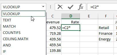
Excel will open the Function Arguments dialog for the VLOOKUP function. Click into the Lookup_Value box and then click on cell B2. Tab to the Table_Array box. Select cells F2:R4 using the mouse and then press the F4 key to add four dollar signs to the range address.
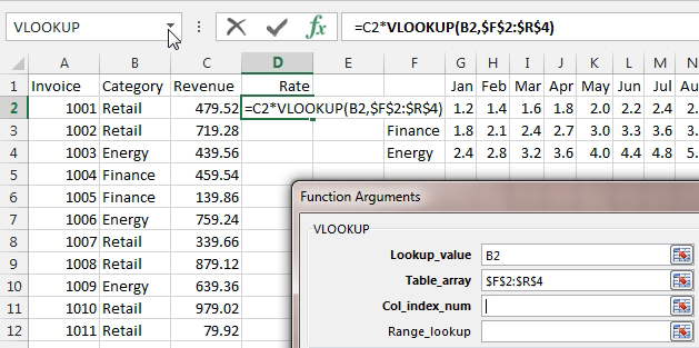
Press Tab to move to the Col_Index_Number argument. This is where you want the MATCH function to appear, so open the Name Box again and choose MATCH from the list. The Function Arguments dialog will switch over to help you build the MATCH function. The formula in the Formula Bar will continue to show the formula in progress, including the VLOOKUP function, but the Function Arguments dialog is now focused strictly on MATCH.
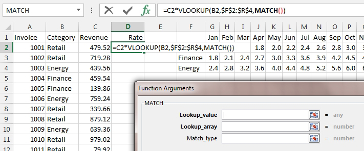
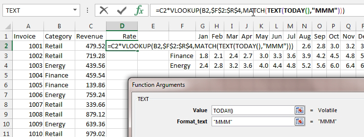
In the MATCH function, you want a lookup value that represents the current month name. This can be achieved with TEXT(TODAY(),“MMM”). While the flashing cursor is in the Lookup_Value box, open the Name Box and choose TEXT. The Function Arguments dialog switches over to show the arguments required for TEXT. The formula bar continues to show the complete formula with VLOOKUP and MATCH.
The TODAY function requires no arguments, so you can simply type TODAY() as the Value argument. Press Tab to move to the Format_Text box and type “MMM” to indicate the desired format.
AVOID CLICKING OK
Since you are done with the TEXT function, it would be tempting to click OK, but that would lead to an error. You can only press OK when the entire formula is complete. Somehow, you need to return back to the Function Arguments dialog for the MATCH formula that is still in progress. Using the mouse, hover over the word MATCH in the Formula Bar and click. Excel will return back to the MATCH version of Function Arguments. Press Tab to move to the Lookup_Array. Select cells G1:R1 using the mouse and press F4 twice to add dollar signs before the row numbers. Tab to Match_Type and type a zero to specify an exact match.
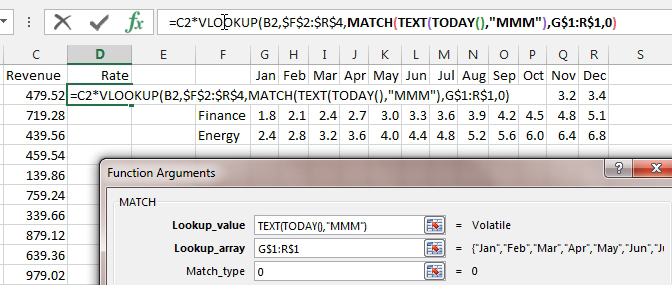
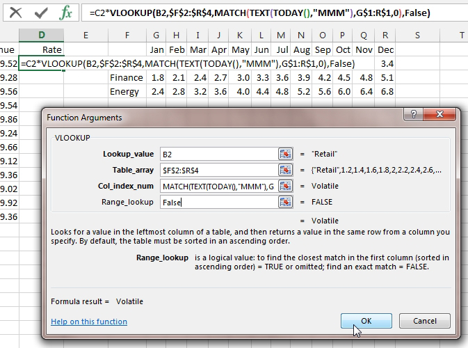
The formula still isn’t complete. Hover over the word VLOOKUP in the formula bar and click to return to the VLOOKUP version of Function Arguments. The first three arguments will be filled in. Tab to Range_Lookup and type FALSE. Since the formula is complete, you can now click OK to close the Function Arguments dialog and enter the formula.
EDITING AN EXISTING FORMULA USING FUNCTION ARGUMENTS DIALOG
Now suppose that at some point in the future, a coworker admires your formula but wonders why you used MATCH and TEXT functions when it would have been convenient to use MONTH(TODAY()). When evaluated during the month of May, this formula fragment would return 5 since May is the fifth month. Simply add 1 to specify that the May data is coming from the 6th column in the lookup table. Carefully replace the word MATCH with MONTH in the formula bar. While the flashing cursor is touching the word MONTH, click the fx icon to the left of the formula bar.

Excel will open the Function Arguments dialog for the MONTH function.
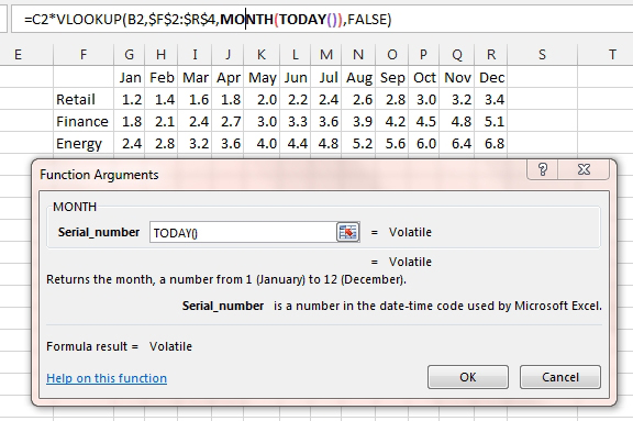
After typing TODAY() in the Serial_Number field and clearing out the remaining arguments left over from the MATCH function, you need to add 1 to the result of the MONTH function. Using the mouse, click just after the closing parenthesis for the MONTH function. Feel free to ignore the VLOOKUP version of Function Arguments while you continue typing +1 in the Formula Bar.
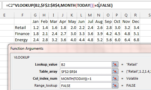
Press Enter or click OK to accept the new formula.

The Function Arguments dialog is a very useful way to learn about each of the arguments in any function that might be new to you. Using the methods described in this article, you can now successfully use the dialog when you have to nest several functions inside of each other.
SF SAYS
Avoid the temptation to click OK before the entire formula is complete.

May 2017


