

Sorting used to be easy in VBA. You would specify up to three key fields and indicate if you wanted each field sorted ascending or descending. But following the release of Excel 2007, sorting became complicated. You can now sort by cell color, font color, or icon, and you’re allowed more than three levels. Yet even if you’re doing a simple “Sort by column F descending within column C ascending” sort, the macro recorder generates complicated code that could allow for sorting by color or icon. Unfortunately, that recorded code also remembers that you had 123 rows, even if you have more or less rows in the future. Let’s look at a way to use the old sort method in Excel 2007 or later versions.
CAVEATS FOR THE OLD SORT METHOD
The sort method used in this article doesn’t allowing sorting by color or by icon. Your data needs to have a single row of headers at the top. If there are titles above the headers, a blank row is needed between the titles and headers. For example, if you have titles in cells A1:A3, then row 4 needs to be completely blank. The same applies if you have boilerplate notes below the data—there has to be a completely blank row between the last row of data and the notes. And if you have some tables to the right of the data, you need one completely blank column between your data and the other tables.
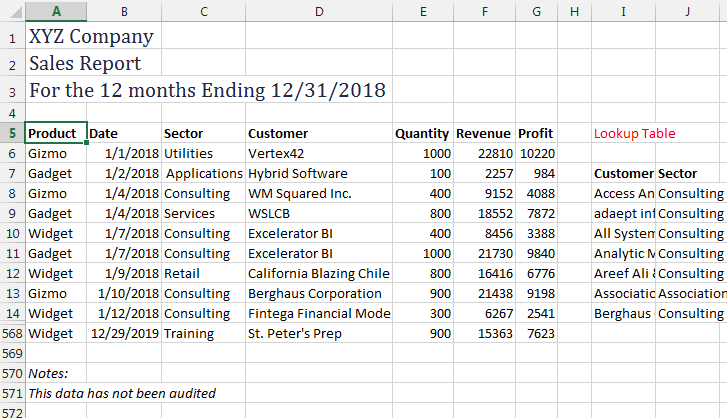
In Figure 1, there is a blank row (row 4) between the titles and headings. A blank row 569 separates the main data set from some explanatory notes. A blank column H separates the main data set from a lookup table in columns I and J. And row 5 is the the single row of headings.
USING CURRENTREGION
When you choose a cell in any data set and click the sort buttons, Excel expands the selection to include the current region, which is all of the data surrounding the active cell in all four directions—it stops at any edge of the worksheet or any completely blank row or column. To see the current region, choose one cell in the data set and press Ctrl+*. In Figure 1, the current range is cells A5:G568. Putting the cursor on any one of those cells and pressing Ctrl+* will result in Excel selecting all the cells from A5 to G568.
In VBA macros, you can use the CurrentRegion property to expand a selection to include the current region. If you routinely have data that starts in A5:G5 but can be any number of rows tall, using Selection.CurrentRegion.Sort will sort all of the data starting at cell A5 and ending at column G in the last row with data.
TYPING THE MACRO
Press Alt+F11 to access the VBA Editor. If you have already recorded a macro, you can find the lines related to sorting and replace them with the code. If you plan on typing the macro without using the macro recorder, you can choose Insert, Module from the VBA menu.
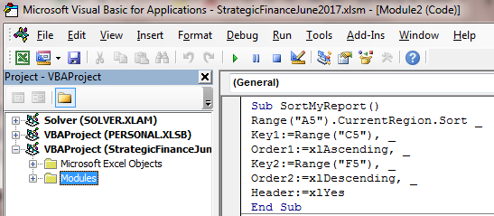
In the macro (below and in Figure 2), each line ends with a space and an underscore. These two characters are known as a continuation character. The sorting method happens in a single line of code, but will be shown as six lines:
Sub SortMyReport()
Range(“A5”).CurrentRegion.Sort _
Key1:=Range(“C5”), _
Order1:=XLAscending, _
Key2:=Range(“F5”), _
Order2:=XLDescending, _
Header:=XLYes
End Sub
The first line, Sub SortMyReport(), gives the macro a name. If you want to assign the macro to an icon on the Quick Access Toolbar, find its name in the list of macros.
The second line, Range(“A5”).CurrentRegion.Sort, tells Excel that you want to select cell A5 and sort the current region.
Key1 identifies the column that will be the primary sort column. Order1 is the direction of the sort. Note that the choices are XLAscending or XLDescending—the first two characters in both are the letters X and L, not an X followed by the number 1. Key2 is the column for the secondary sort. The macro uses the Revenue heading in cell F5 and specifies that Excel should sort descending. If you wanted to include a third sort level, you would add a new pair of lines specifying Key3 and Order3.
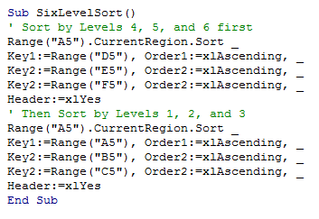
What if you need to do four, five, or six levels of sorting? You aren’t allowed to specify Key4. But you could have a macro that does two sorts. The first sort should be by fields 4, 5, and 6. The second sort should be by fields 1, 2, and 3.
The Header line tells Excel that you have a single row of headers. Excel usually guesses if your data has headers and frequently guesses wrong. Your choices for header are XLGuess, XLYes, or XLNo. Always specify either XLYes or XLNo since the guessing algorithm in VBA is just as likely to be wrong as in the Excel interface.
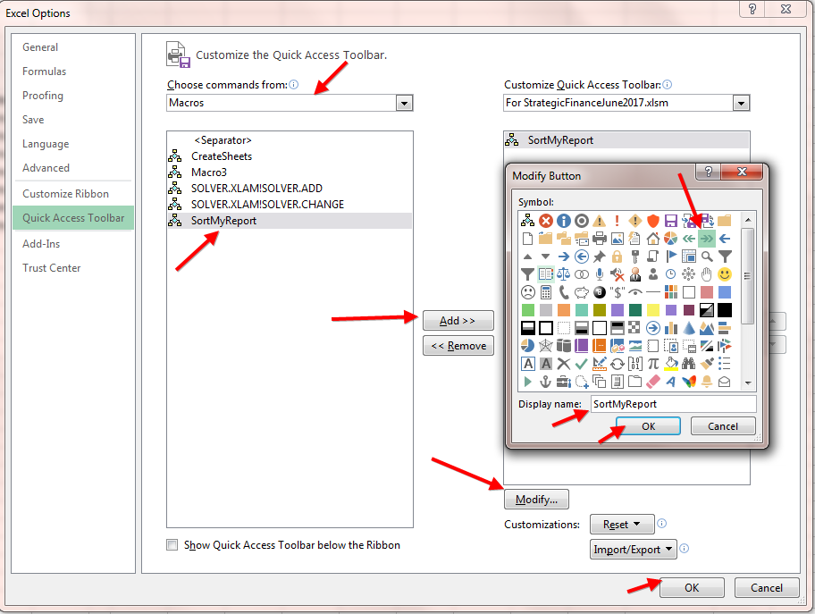
To assign a macro to an icon in the Quick Access Toolbar, follow these steps:
- Right-click the Quick Access Toolbar and choose Customize Quick Access Toolbar.
- From the top-left dropdown, select Macros. (It defaults to Popular Commands.)
- In the top-right dropdown, which defaults to For All Documents, select the option that indicates it’s for this particular workbook. For example, if the file was named XYZCompany.xlsx, the choice “For XYZCompany.xlsx” would be available.
- Select SortMyReport in the left box and click the Add >> button in the center of the screen to add it to the list in the box on the right.
- In the right-hand box, select SortMyReport. Click the Modify button at the bottom-right of the dialog.
- Choose a new cell icon and type some ToolTip text to appear by changing the Display Name.
- Click OK to close the Modify Button dialog. Click OK to close the Excel Options dialog.
To watch a video of these steps, go to www.youtube.com/watch?v=Qu542zr1cZ8.
Adapting this simple macro to your data set will allow you to quickly perform common multiple-level sorts.

June 2017

