FOR CALENDAR YEARS
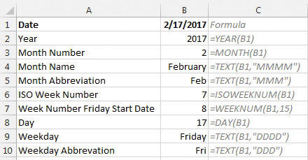
If your financial year ends on December 31, then you can use a short formula. (Figure 1 shows the Excel functions that you can use to convert a date into years, months, weeks, or weekdays.) First, use the =MONTH() function to convert the date to a month number. Divide that result by 3. Dates in January will return 0.33, February 0.67, March 1.00, April 1.33, and so on. By using the =ROUNDUP() function, you will have 1 for January, February, and March; 2 for April through June; and so on.
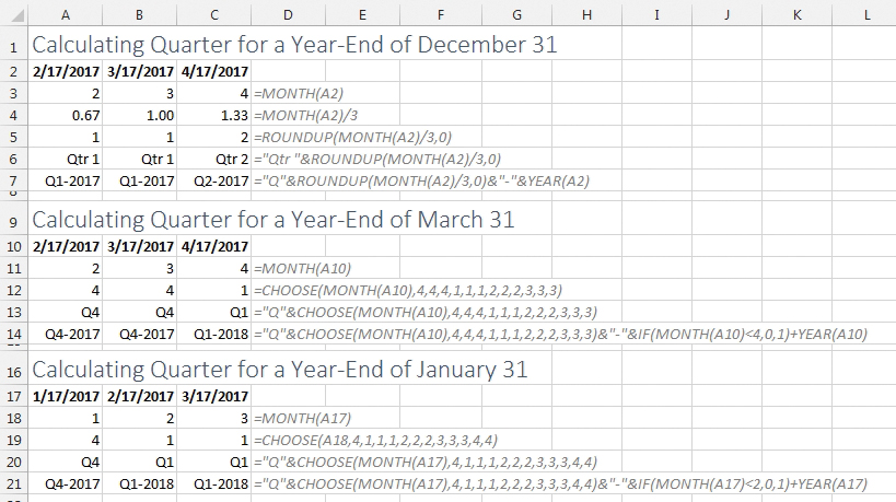
To show the quarter as “Q1” or “Qtr 1,” concatenate the appropriate text before the result. In Figure 2, cell A7 uses a formula of =“Q”&ROUNDUP(MONTH(A2)/3,0)&“-”&YEAR(A2) to return “Q1-2017.”
FOR OTHER FISCAL YEARS
Fiscal years ending January 31 are common in retail companies. Government contractors might use a fiscal year end of September 30. To calculate a fiscal quarter, first convert the date to a month number using =MONTH(). This result is limited to 12 integers from 1 to 12.
You could use a VLOOKUP formula to convert month number to quarter number. But the formula =VLOOKUP(MONTH(A2),{1,4;2,1;5,2;8,3;11,4},2) is difficult to remember and type. The array constant inside the curly braces holds a 5-row by 2-column lookup table.
Instead, the =CHOOSE() function would let you specify 12 quarter numbers that correspond to months 1 through 12. If your fiscal year ends in January, you would use =CHOOSE(MONTH(A2),4,1,1,1,2,2,2,3,3,3,4,4). For a fiscal year ending in March, use =CHOOSE(MONTH(A2),4,4,4,1,1,1,2,2,2,3,3,3).
If you would prefer to show the quarter as Q1 instead of 1, you can use the ampersand to concatenate a “Q” before the CHOOSE function. The results are shown in cells A13 and A20 of Figure 2, with the formulas shown in D13 and D20.
APPENDING A FISCAL YEAR TO THE QUARTER
In some companies, the fiscal year is determined by the calendar year in which the 12th month of the year occurs. For example, a fiscal year that runs from February 2017 to January 2018 would have quarters called Q1-2018 through Q4-2018. In other companies, the fiscal year might be referred to as something like “17-18.”
For the case where the fiscal year is the year of the ending month, use an IF() function to test if the month number is less than the starting month. For example, with a fiscal year ending in January, the fiscal year will be =YEAR(A2) if the date is before February and =YEAR(A2)+1 in February and later. Thus, to include the fiscal year with the quarter, you could use =IF(MONTH(A2)<2,0,1)+YEAR(A2).
For a year ending in March, you would change the <2 test to be <4: =IF(MONTH(A2)<4,0,1)+YEAR(A2). For a year ending in September, you would test for <10: =IF(MONTH(A2)<10,0,1)+YEAR(A2).
Cell A21 in Figure 2 shows how to concatenate the fiscal quarter and year together using this long formula: =“Q”&CHOOSE(MONTH(A17),4,1,1,1,2,2,2,3,3,3,4,4)&“-”&IF(MONTH(A17)<2,0,1)+YEAR(A17). That would return the quarter in a format of “Q4-2017.”
If, instead, you need it to say 17-18, the long formula becomes even longer. Just to get the year portion of the formula, you would use: =IF(MONTH(A2)<4,MOD(YEAR(A2)-1,100)&“-”&TEXT(A2,“YY”),TEXT(A2,“YY”)&“-”&MOD(YEAR(A2)+1,100)).
RETURNING A PERIOD INSTEAD OF A MONTH
I recently conducted a seminar for IMA® in Nashville. Because the Tennessee state government has a fiscal year ending in June, they preferred to report using a period number instead of a month. July is period 1, December is period 6, January is period 7, and so on. In this case, a lot of the coworkers used a VLOOKUP table off to the right side of the data. But they also could use =CHOOSE(MONTH(A2),7,8,9,10,11,12,1,2,3,4,5,6) to achieve the same result.
DATES CAN'T BE TEXT
The caveat for all of these formulas is that you are storing your dates as real dates and not as text. A quick way to check: Press Ctrl and the Grave Accent key (`) to toggle into Show Formulas mode. Real dates will convert to a serial number such as 42783. If you still see a text date, the formulas won’t work. Press Ctrl+` again to exit Show Formulas.
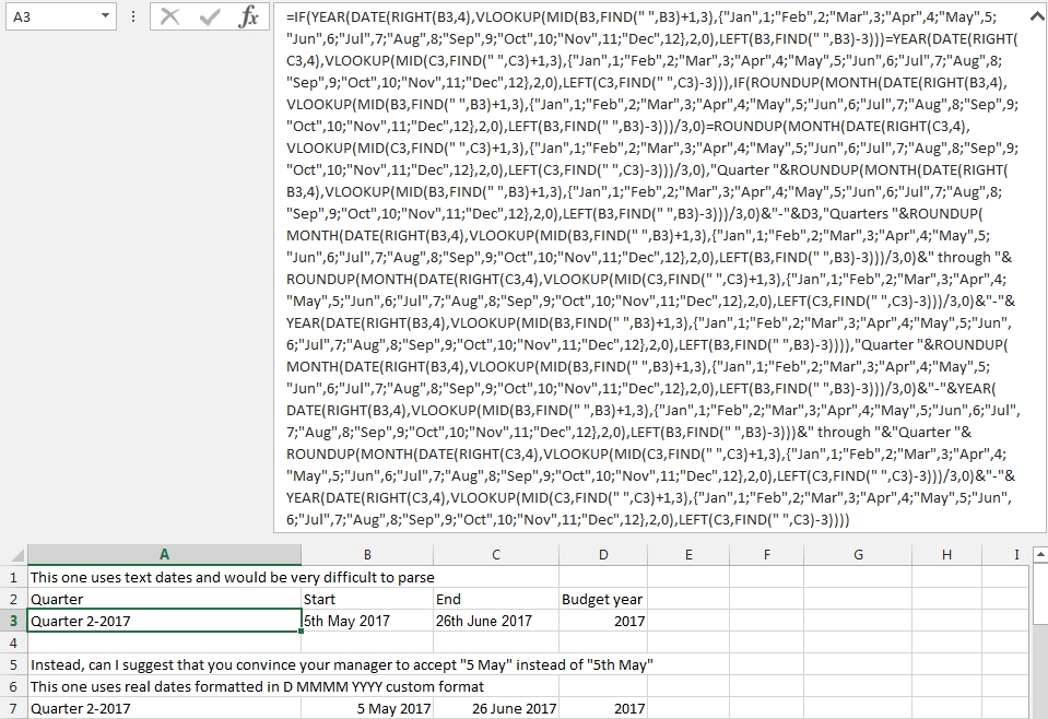
I recently ran across a worksheet in which the manager wanted dates to display as 1st Feb 2017, 2nd Feb 2017, 3rd Feb 2017, 4th Feb 2017. The suffixes after the date (“st,” “nd,” “rd,” and “th”) convert a cardinal number to an ordinal number. While the Excel Fill Handle will allow you to create a column of cardinal numbers easily, the formulas in this article become far more complex. A 41-character formula grew into 2,438 characters in order to handle the text dates (see Figure 3).
SF SAYS
Many formulas that reference dates will change the cell format to a date. Plan on formatting this month’s formula cells as numeric.

February 2017


