Excel: Creating Tables from Timeline Slicers

December 01, 2017

Slicers are visual tools that filter one or more pivot tables in a workbook. Regular slicers debuted in Excel 2010, and Excel 2013 saw the introduction of the Timeline slicer, which can only be applied to dates. A dropdown menu on the slicer lets you filter by year, quarter, month, or day. The bottom portion shows the date range selected.

I’ve never been a fan of Timeline slicers. Say you have one showing months and select September through October. If you switch to show quarters, the slicer will attempt to illustrate those parts of Q3 and Q4 that are selected, i.e., September through October (see Figure 1). Unless you notice the “Sep–Oct 2017” at the top of the slicer, it’s difficult to interpret the slicer. Nick, an IMA® member from Utah, asked if there’s a better way to show the dates selected. By using a disconnected pivot table, you can create a useful title for your worksheet that shows the days or months selected.

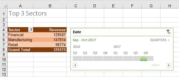
Consider a pivot table that shows the top three sectors from a data set. With one cell in the original pivot table selected, choose Analyze, Insert Timeline. In the Insert Timelines dialog, choose your Date field and click OK. At this point you’ll have a single pivot table associated with a timeline, as shown in Figure 1.

DISCONNECTED PIVOT TABLE

Here are the steps to copy the original pivot table into a disconnected pivot table that will be used with a formula to create the title for your report:

Select the entire original pivot table (cells A4:B8).
Press Ctrl+C to copy the pivot table.
Select a cell outside of your print range, such as cell L4, and press Ctrl+V to paste. You’ve now created a second pivot table that’s automatically connected to the Timeline slicer. (Using the copy and paste method is crucial. If you insert a new pivot table instead, it won’t be connected to the existing slicer.)
With the second pivot table selected, remove all fields from it.
Drag the Date field from the top of the Pivot Table Fields list to the Values area at the bottom of the Pivot Table Fields list. Oddly, the pivot table will default to a Count of Date.
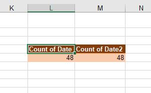
Drag the Date field a second time to the Values area, giving you two columns in the pivot table: Count of Date and Count of Date2. (See Figure 2.)
Double-click the heading for Count of Date to open the Field Settings dialog for that column. Change the calculation from Count to Min. Change the Custom Name to “From.” Click OK to close the dialog box. (See Figure 3.)

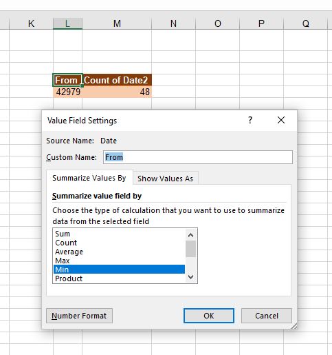
Double-click the heading for Count of Date2 to open that column’s Field Settings dialog. Change the calculation from Count to Max. Change the Custom Name to “Through.” Click OK to close the dialog box.

You will now have an odd-looking four-cell pivot table that says something like From 42979 Through 43039. While the numbers 42979 and 43039 don’t look like dates, they are date serial numbers. If you select those numbers and apply a number format of Short Date, the dates will appear.

BUILDING A FORMULA

In general, be careful when you build a formula pointing to a cell in a pivot table. You need to type the cell references directly rather than selecting the cell with the mouse or arrow keys. Using the mouse or arrow keys will insert =GETPIVOTDATA() functions instead of the cell reference.

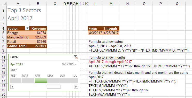
The formula to generate the title will vary depending on the date format you want to display. For a title that includes a date range format such as “March 1, 2017 - April 28, 2017,” enter the formula =TEXT(L5, "MMMM D, YYYY")& " – "&TEXT(M5,"MMMM D, YYYY") in cell A2 (or wherever you want the title to appear). The Timeline slicer is asking for dates in March and April. The underlying data set contains invoices that are issued on most weekdays. Because April 1, 2, 29, and 30 fell on weekends, there were no invoices for those dates. Therefore, the end date shows as April 28 instead of April 30.

To use a format such as “March 2017 through April 2017,” as shown in Figure 4, use the formula =TEXT(L5, "MMMM YYYY")& " through "&TEXT(M5,"MMMM YYYY"). This formula is fine when two or more months are selected, but if you only choose one month, you’ll end up with a title like “April 2017 through April 2017.”

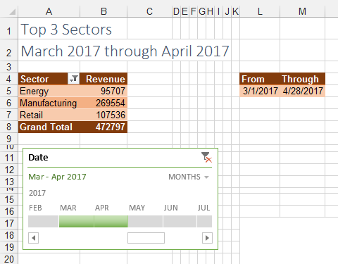
To create a formula that looks good even when a single month is selected, use: =IF(TEXT(L5,"MMMM YYYY")=TEXT(M5,"MMMM YYYY"),TEXT(L5,"MMMM YYYY"),TEXT(L5,"MMMM YYYY")&" through "&TEXT(M5,"MMMM YYYY")). When only one month is selected, the formula will then switch to a title like “April 2017” (see Figure 5).