CALCULATING A UNIQUE RANK
In Figure 1, a series of RANK functions in column A is attempting to rank 10 salespeople. Harry (row 9) is in first place with $550. But the RANK function encounters a tie for second place. Both Andy (row 2) and Flo (row 7) have $540. Excel doesn’t want to play favorites, so it assigns a rank of 2 to both. No one will be ranked third. The next sales rep is Jill in fourth place (row 11). You’ll see other ties for sixth place and eighth place, meaning that no one is ranked seventh or ninth.
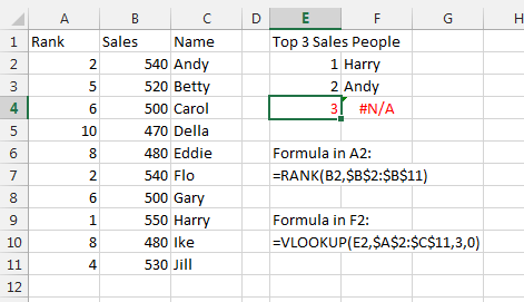
While this method of handling ties might be fair, it can cause problems if you’re trying to figure out the top three salespeople using VLOOKUP formulas, as shown in cells E2:F4. VLOOKUP doesn’t realize that two people are ranked second. Andy is reported as the second best rep, and no one is ranked at number 3.
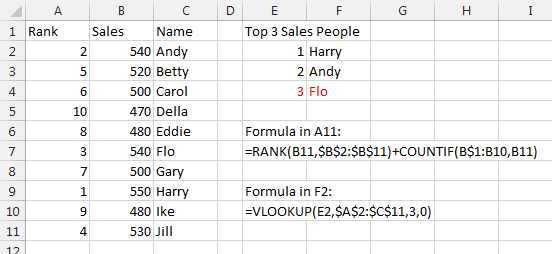
The common workaround is to build a formula that calculates both a RANK and a COUNTIF of how many times the current rep’s exact sales amount is found above the current rep. For example, if you used a formula of =RANK(B10,$B$2:$B$11)+COUNTIF(B$1:B9,B10) in cell A10 for Ike, you would get 8 as the rank and 1 as the count of records above Ike that had exactly $480. Thus, Ike would be ranked ninth and Eddie would be ranked eighth, as in Figure 2.
THE UNIQUE RANK FORMULA STOPS WORKING
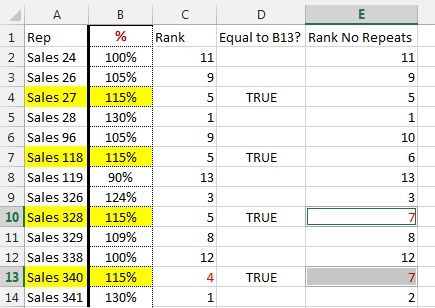
Recently, someone came to the MrExcel.com message board with a situation where the unique rank formula was returning abnormal results. Out of a list of 13 sales reps, two people were being ranked seventh and no one was ranked fourth. This isn’t supposed to happen. In Figure 3, both cells E10 and E13 are reporting a rank of 7.
After downloading the workbook, I could see that the RANK function was applied to a column of percentages. Four sales reps were tied at 115%. Each of the four cells showed 115%. Even when I pressed Ctrl+` to see the underlying values, those four cells continued to show 115% (see Figure 4).
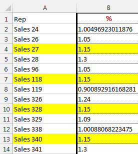
I tested that each of the 115% values were equal to each other with simple formulas such as =B4=B13. I tested how many 115% values were seen by COUNTIF, and the answer was 4. Everything was telling me that those four sales reps had exactly 115%. I even used VBA to inspect the cells, and they all contained 115%.
But then I tried sorting the data descending. If those four sales reps were truly tied at 115%, they should appear in the sorted data in the same order as in the original data. Strangely, though, the fourth sales rep with 115% moved above the others (see Figure 5). Something was happening behind the scenes.
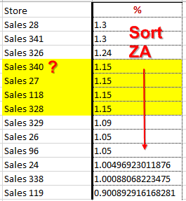
17 DIGITS OF PRECISION
I sent the worksheet to Microsoft’s Excel team in Redmond, Wash. When they looked in the XML, they noticed that three of the sales reps didn’t have 1.15. Those three reps had 1.49999999999999999. Even though Excel is only supposed to use 15 digits of precision, these cells contained 17 digits of precision. Everything in Excel that was designed to work to 15 digits of precision was rounding the 16th and 17th digits up and calculating as if the cell contained 115%.
But, inexplicably, the sorting algorithm and the RANK function were making use of all 17 digits. This breaks rules that hard-core Excel users have relied on for decades.
Theoretically, the Excel team is in a quandary with this problem: Rewriting RANK and Sort to respect the 15-digit limit would slow all of Excel down. Rather than provide a slower experience to 749,999,999 other people, the individual with the four apparently identical 115% cells is considered an edge case that’s going to simply break Excel.
But in real life, others will inevitably have this problem with RANK. If you’re ever using RANK with numbers that are the result of a division with several decimal places, you might be affected. One simple workaround would be to round your results off to 14 digits to make sure that you never get stung by the secret 16th and 17th decimal place: =ROUND(A2/B2,14).
SF SAYS
Those tiny differences in the 16th and 17th digits after the decimal can lead to unexpected formula results.

August 2017


