ADDING UNFORMATTED SUBTOTALS
Say that your data has Account Number (such as A1001, A1002, etc.) in column A, Description in column B, and Amount in column C. Make sure to sort the data by Account Number so that all of the rows for each account appear in adjacent rows.
From the Data tab, select Subtotals. In the Subtotal dialog box, the default settings assume you want to use the Sum function to add a subtotal to the right-most column (in this case, column C) at each change in the first column. But if you have extra columns in the data, you might need to adjust the settings to choose Sum and the correct columns.
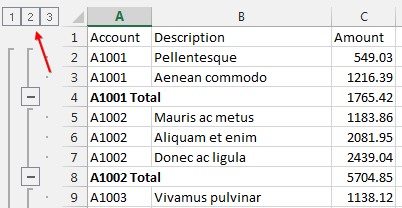
Click OK in the Subtotal dialog, and Excel will insert new subtotal rows in the data. New Group and Outline buttons also will appear to the left of column A. The #2 button will collapse the data and show only the subtotals and grand total.
FORMATTING SUBTOTALS
The Subtotal command will bold the words “A1001 Total” in column A, but no special formatting gets applied to the numbers in column C.
Click the #2 Group and Outline button to see only the subtotal and grand total rows. Select the numbers in column C.
At this point, any formatting you add will be applied to both the numbers that you can see and the numbers in the hidden rows. Since your goal is to format only the subtotal rows, you need to use the Visible Cells Only command.
The long way to find this command is Home, Find & Select, Go To Special, Visible Cells Only, OK. Alternately, simply press Alt+; as the shortcut.
It’s important to select Visible Cells Only correctly. If you continue the next steps without selecting the visible cells, all of the detailed rows will be formatted along with the subtotal rows.
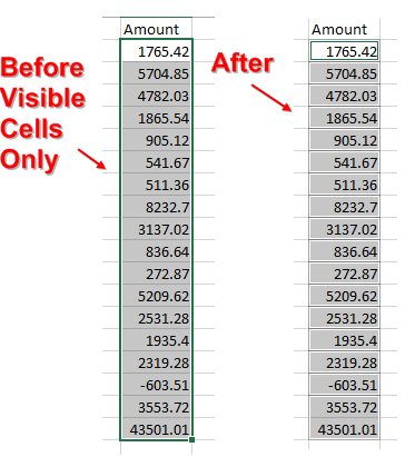
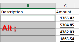
Look for a change in the selection rectangle after you’ve applied Visible Cells Only (or pressed the shortcut). Before, there was a single border around the selection. The active cell is white, and the remaining cells in the selection are a single block of gray fill.
After Visible Cells Only is selected, the active cell has a thin border. The other cells in the selection are gray, but thin white lines surround each cell (or group of cells, in the case of the last subtotal and the grand total).
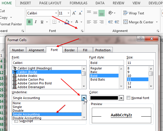
Apply bold formatting to the subtotals using Ctrl+B. To apply a Single Accounting Underline, open the Format Cells dialog and go to the Font tab. (Either right-click the cell and select Format Cells and then navigate to the Font tab, or click the dialog launcher in the Font group of the Home tab of the ribbon to open the Format Cells dialog directly on the Font tab). Open the Underline dropdown and choose Single Accounting. Click OK.
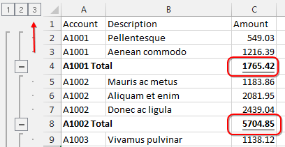
To check the formatting, click the #3 Group and Outline button and check that each of the subtotals is in bold text and have accounting underlines.
Select the Grand Total cell and apply a Double Accounting Underline to that cell.
SHIFTING SUBTOTALS RIGHT
To shift the subtotal formulas to the right, you need to select the blank cells to the left of each subtotal. Click the #2 Group and Outline button. Select the range of blank descriptions in column B.
Press Alt+; to select only the visible rows. Again, look for the thin white lines appearing between each block of gray in the selection area to confirm that you have successfully selected only the visible cells. Don’t continue with the next steps if you don’t see the thin white lines. (If Alt+; isn’t working for you, try Home, Find & Select, Go To Special, Visible Cells Only, OK.)
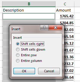
At this point, you could insert new cells and shift cells to the right. Go to Home, Insert, Insert Cells…, and choose Shift Cells Right in the Insert dialog. Figure 2 shows the final results.
Click the #3 Group and Outline button. The subtotal rows have moved from column C to column D. Select one of the subtotal cells, and you’ll see that the formula in column D correctly points back to the numbers in column C. This behavior is similar to a Cut and Paste where the pasted cells keep pointing back to the original range. But in this instance, a Cut and Paste would have the formulas in column D pointing to blank cells in column D, which wouldn’t work.

November 2016


