FROM FOLDER
If you have Excel 2016, use Data, New Query, From File, From Folder. In Excel 2010-2013, download the free Power Query add-in from Microsoft, then use Power Query, From File, From Folder. In either version, you will be asked to browse to the folder containing the CSV files.
This will take you to an Excel-like grid listing all of the files in the folder and any subfolders. Use the Filter dropdown at the top of the extension column and uncheck any files you don’t want to include, especially all the non-CSV files (such as the Thumbs.db file that Windows often adds to a folder).
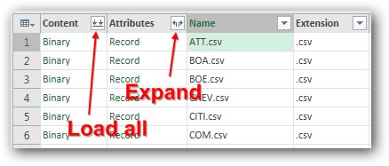
Columns in the grid include file name, date accessed, date modified, date created, and folder path. Two cryptic columns also appear. The Content column says “Binary” in each row. The Attributes column says “Record” in each row. If you click the expand icon (the two-headed arrow) next to the Attributes heading, you can choose to show additional fields, such as file size.
But the amazing icon is shown next to the Content column in Figure 1. When you click the icon with two down arrows, Excel will load all of the records from all of the CSV files in the grid.

POWER QUERY
If you use this technique to load 200 CSV files into the grid, you might find that the header row appears 200 times in the file. The header row from the first file is the only one you need to keep. All of the others have to be deleted. This is fairly easy in Power Query.
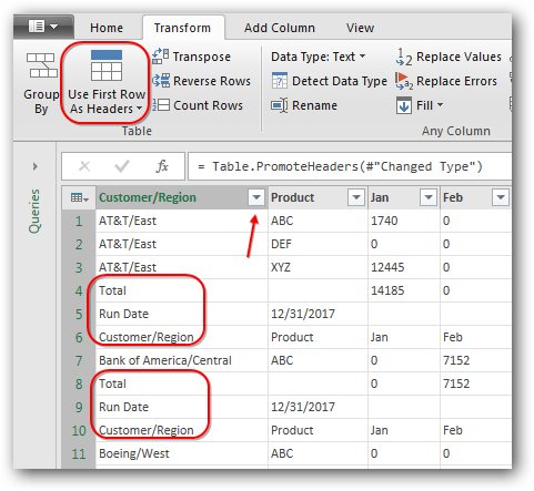
First, choose the Transform tab and click Use First Row As Headers. This promotes the first row from the first CSV file to be field names.
To remove the other headers, you can open the Filter dropdown in the first column and uncheck certain values. In Figure 2, use the Customer/Region dropdown to remove any rows that have Customer/Region. In the example here, you would also uncheck any values that say Run Date or Total so you’re left with only the data rows from each file.

Once you have only the data records, you can use other Power Query tools such as Split Column and Unpivot to further clean the problems in the file. For a video demonstration of the remaining steps to clean this data, watch the video below.
RETURNING DATA TO EXCEL
Once you clean the data in Power Query, use the Home, Close & Load command to return the complete set of records to your Excel workbook.
If your complete set of records ever extends past the 1,048,576 rows in Sheet 1, you can use the Close & Load dropdown to choose the Close & Load To… command. Choose Add Data to the Data Model and Connection Only. You can then use Pivot Tables to report from the results of the query. After choosing Insert, Pivot Table, choose Use This Workbook’s Data Model in the Create PivotTable dialog.
NEW OR UPDATED CSV FILES
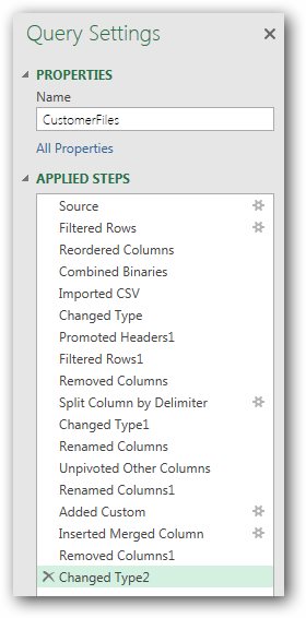
Here is where Power Query really shines. Although originally loading the data was faster using Power Query, the amazing part is that Power Query uses the M programming language to record all of the data cleansing steps and stores them with the query definition (see Figure 3).

If new CSV files are added to the folder, you can open the original workbook and use the Refresh icon on the Workbook Queries pane to have Power Query repeat all of the steps in loading the data. For that annual budget consolidation process that I mentioned in the first paragraph, it would take an entire day to do the first combine, and replacing or adding new files would take minutes. Using Power Query, the initial combine takes 10 minutes, while replacing or adding new files becomes a single click on Refresh and a few seconds of processing.
A FOLDER OF EXCEL FILES?
As I write this, the ability to combine a folder of Excel files isn’t available in Power Query. Unlike CSV files, the data in Excel files can be spread across multiple sheets, so the process is more difficult. Microsoft will eventually add this feature. In the meantime, a small macro to save your Excel files as CSVs would allow you to use Power Query.

January 2016


