Excel: Shortening a VLOOKUP

A BUNDLED MESS

The creator of this worksheet used formulas to pull data from 20 other worksheets into one monolithic worksheet so it could be fed into a single pivot table. The formulas worked but weren’t efficient. For example, in order to populate columns called Quota Jan, Quota Feb, Quota Mar, through Quota Dec, the formula used 12 separate nested IF statements. Note the portions in blue are changing the lookup column returned by VLOOKUP:

=IF(MONTH(C2)=1,VLOOKUP(A2,Quotas!$A$1:$M$9999,2,False),
IF(MONTH(C2)=2,VLOOKUP(A2,Quotas!$A$1: $M$9999,3,False), IF(MONTH(C2)=3,VLOOKUP(A2,Quotas!$A$1: $M$9999,4,False), IF(MONTH(C2)=4,VLOOKUP(A2,Quotas!$A$1:$M$9999,5,False),
IF(MONTH(C2)=5,VLOOKUP(A2,Quotas!$A$1:$M$9999,6,False),
IF(MONTH(C2)=6,VLOOKUP(A2,Quotas!$A$1:$M$9999,7,False),
IF(MONTH(C2)=7,VLOOKUP(A2,Quotas!$A$1:$M$9999,8,False),
IF(MONTH(C2)=8,VLOOKUP(A2,Quotas!$A$1:$M$9999,9,False),
IF(MONTH(C2)=9,VLOOKUP(A2,Quotas!$A$1:$M$9999,10,False),
IF(MONTH(C2)=10,VLOOKUP(A2,Quotas!$A$1:$M$9999,11,False),
IF(MONTH(C2)=11,VLOOKUP(A2,Quotas!$A$1: $M$9999,12,False), IF(MONTH(C2)=12,VLOOKUP(A2,Quotas!$A$1:$M$9999,13,False)))))))))))).

This massive formula was trying to detect which column of a VLOOKUP table to return. Based on the date in column C, the IF statements were translating to a month number, and then choosing which column to return from the lookup table. Remember, there were 60,000 rows times 12 columns of this large formula. That’s 720,000 VLOOKUP formulas looking into a table with 10,000 rows.

It would be simpler to have a single VLOOKUP formula and have some logic inside of the third argument to decide which column to return. In this particular case, the logic for the third argument amounted to the month number of the date found in C2 plus 1. You could simplify the formula to: =VLOOKUP(A2,Quotas!$A$1:$M$9999,MONTH(C2)+1,False).

What if the conversion isn’t that simple? What if you were trying to use a region name in column D to find a particular column in a lookup table? If the headings in the lookup table contain the exact same region names found in the heading row of the table, you could use a MATCH formula to return the correct column number: =VLOOKUP(A2,RegionTable!$A$1$P$9999,MATCH(D2,RegionTable!$1:$1,0),False).

But even these solutions would leave 720,000 VLOOKUP formulas. You’re still going to have very slow recalculation times.

Further, the resulting pivot table was horribly malformed. This analyst resorted to adding the 12 Quota fields to the Rows area so they appear in the pivot table. Any time that you have 12 columns showing quota (or any number) for each month, you can build a better pivot table by unpivoting the original data. The new Power Query tool from Microsoft makes unpivoting a few clicks.

NO MORE FLATTENING DATA

In the past, data for a pivot table had to be in one place. Starting in Excel 2013, you can easily create pivot tables from separate tables. Before you create the pivot table, follow these simple rules for your main data and for each lookup table:

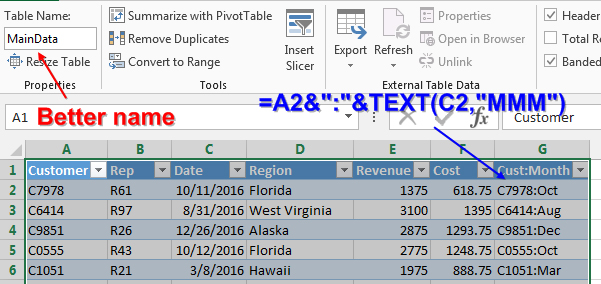
1. Select each data set and press Ctrl+T. This defines the data set as a table. Go to the Table Name field on the Table Tools Design tab in the ribbon and change the default name (Table1) to something descriptive.
2. Make sure there is a single column in your table that will relate to a single column in another table. In Figure 1, column G is a new column that concatenates customer number and month name in order to create a single-column link to a lookup table.



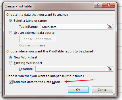
3. Create a pivot table from the main data table. Use Insert, Pivot Table. In the Create Pivot Table dialog box, choose the box for Add This Data To the Data Model. (See Figure 2.)



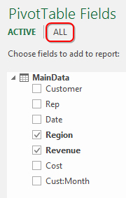
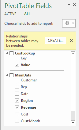
4. The Pivot Table Fields pane will show columns from your original table, but an extra line near the top of the table gives choices of ACTIVE or ALL. (See Figure 3.) Choose ALL, and you can now choose from any of the tables in the workbook. The first time that you choose a field from a new table, the Pivot Table Fields pane will warn you that you need to define a relationship between the tables, as shown in Figure 4.





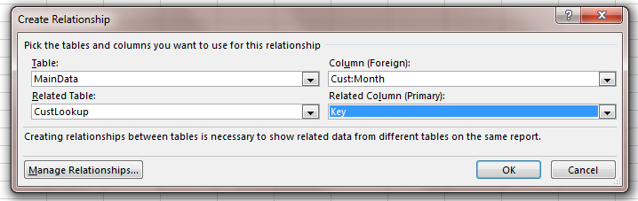
5. Click the Create button and define the single column that can act as a key field between the two tables. (See Figure 5.)

You can now pull fields from various worksheets into the pivot table. If you want months to stretch across the report, you can put the Date field in the Columns area instead of dragging 12 different fields into the pivot table.

CALCULATED FIELDS REQUIRE AN UPGRADE

The ability to join multiple tables in a pivot table first appeared in the Power Pivot add-in for Excel 2010. It’s great that Microsoft incorporated the Power Pivot ability to join multiple tables in Excel 2013 and Excel 2016. Unfortunately, the ability to create calculations between the two tables remained as part of the Power Pivot add-in. That means you have to have Excel 2013 Pro Plus or Excel 2016 Professional to enable the Power Pivot tab to create new calculations. As soon as you need to divide Revenue from the main table by Quota in the lookup table, you will need the more expensive version of Excel to access the calculation features.

SF SAYS

A formula with 12 VLOOKUPs might work, but it can slow recalculation to a crawl. Using related tables instead will resolve the issue and make the worksheet usable.