CREATE A CALENDAR TABLE
Say that you have data for 2016 and 2017 based on the National Retail Federation 4-5-4 Calendar (http://bit.ly/2eCFaae). You need to create a calendar table that has one row for each date in your data set. Add a new worksheet with each day from January 1, 2016, through February 3, 2018, listed in column A. Add columns for year, season, quarter, month, week, day, and weekday. Use row 1 for the header cell for each column. Make sure there are no other heading cells other than those in row 1.
Select one cell in this data set and press Ctrl+T to define it as a table. Confirm that your data has a header row. Excel will apply a default formatting to the table, and a Table Tools Design tab will appear in the ribbon. Look on this tab in the ribbon, and you can see that Excel assigned a name such as “Table1” to the table. Click in the Table Name box and assign a name such as “Calendar.”
Any time that you need to create a pivot table and report using the alternate calendar, you will copy this small worksheet into the workbook containing your sales data.
JOIN MULTIPLE TABLES
You can use Data Model pivot tables to join multiple tables. Say that you have data from your point of sale (POS) system. It includes fields such as Date, Time, Transaction ID, Partner #, Merchandise Amount, Sales Tax, and Total. Even though you could create a pivot table from this data, you need to format the data as a table if you’re going to join it to the Calendar table. Select one cell in the data set and press Ctrl+T. Confirm that the table has headers. Excel will suggest a name such as “Table2.” You should rename the table to something meaningful, like “Sales” or “Transactions.”
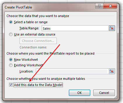
Now go to your transactional data set. Select Insert, Pivot Table. In the Create PivotTable dialog, choose the box for Add This Data to the Data Model.
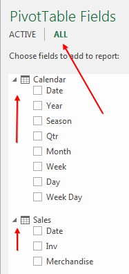
When the Pivot Table Field List appears, there will be a new choice at the top letting you select between Active or All. Change the setting to All, and the Calendar table will appear in the field list as well. Click the triangle icon next to each table to expand the list of fields for each table.
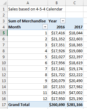
Build a pivot table using fields from the Calendar table in the rows or columns. Place the Revenue field from the transaction table in the Values area.
A yellow box will appear in the Pivot Table Field List showing that Relationships May Be Needed. In Excel 2013, the only choice is Create. In Excel 2016, you can choose to Auto-Detect the relationship. When you choose Create, you have to specify that the Date field from the Sales table is related to the Date field from the Calendar table.
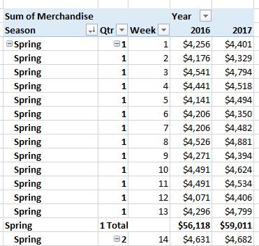
Once you’ve established the relationship, you can build any pivot table using the year, season, quarter, month, week, or weekday fields from the Calendar table.
FILL 4-5-4 MONTH ENDING DATES
While the fill handle is great at filling month names such as January, February, and March, it requires special handling for filling month-ending dates. For a regular calendar, type 1/31/2017 in a cell. Right-click the fill handle and drag. When you release the mouse button, a fly-out menu appears where you can choose Fill Months to make the month-ending dates appear. But there’s no equivalent tool for filling month-ending dates of a 4-5-4 calendar.
Follow these steps:
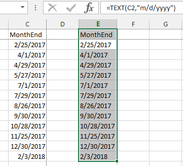
- Type a heading such as MonthEnd and add the month-ending dates to the column.
- In an adjacent column, use =TEXT(C2,“M/D/YYYY”) to convert the dates to text.
- Select your list of text dates and the MonthEnd heading.
- Go to File, Options, Advanced. Scroll most of the way through the list and choose Edit Custom Lists. Click Import to import your list. Click OK.
- In the future, to fill the month-ending dates, type MonthEnd in any cell and drag the fill handle. The text dates will appear. While those dates are selected, type Alt+DEF <enter> to convert the text dates to real dates.

December 2016


