CREATING THE RULES
The attendee had a worksheet with a status code in column D that contains possible values of 1 through 5. Items with a status of 1 should be green, 2 should be blue, 3 yellow, 4 orange, and 5 red. He was also very specific about which shades of blue and green needed to be used.
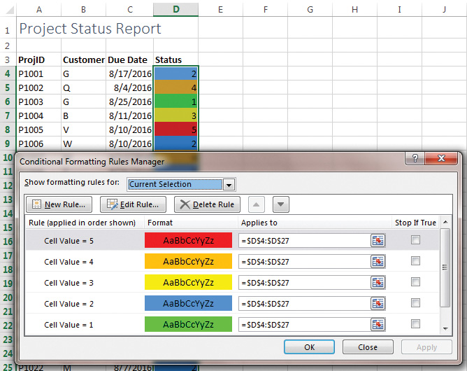
Here are the steps to get the results shown:
1. Select the cells with the status codes.
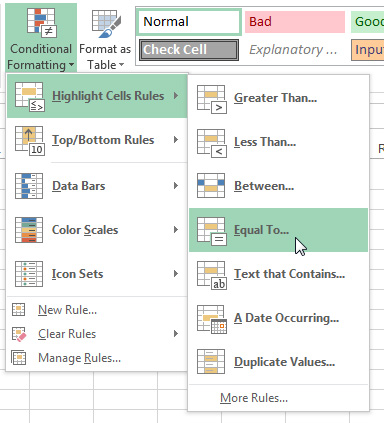
2. On the Home tab, select Conditional Formatting, Highlight Cells Rules, Equal To…
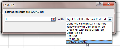
3. In the Equal To dialog box, type a 1 in the left box. Open the dropdown and choose Custom Format…
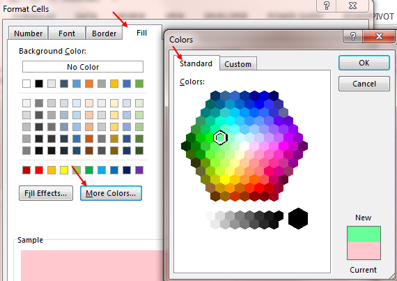
4. The Format Cells dialog opens on the Font tab. You could use this tab to change the color of the numbers in the cell. But to change the fill color of the cell, go to the Fill tab.
5. The 60 available colors have changed with each version of Excel and will change based on the theme used for the document. For a reliable palette of colors, click More Colors. This offers 163 colors, including many shades of popular colors such as red, orange, yellow, blue, and green. But if none of those colors are the exact right shade, you can use the Custom tab to choose from 16.7 million colors.
6. After choosing a color, click OK in each of the three open dialog boxes in order to return to Excel.
7. Repeat steps 2 through 6 for each of the four remaining colors, changing the 1 in step 3 to the other values.
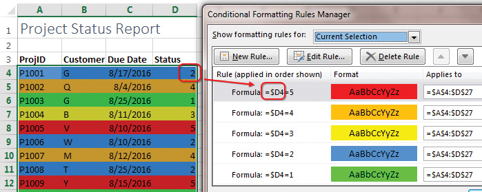
To review the rules, go to Home, Conditional Formatting, Manage Rules.
HIGHLIGHTING THE ENTIRE ROW
Rather than highlighting only the status cell, you might want to highlight the entire row. This is possible using a formula-based condition. In the sample spreadsheet, the first row with data is in row 4, and the status code is in column D. You need to write a formula where the reference to column D is marked as absolute by using a single dollar sign. The reference to row 4 needs to be relative with no dollar sign.
Thus, for the data set, the formula of =$D4=1 would be used to find items that should be green. Use the following steps to get the results in Figure 2:
1. Select the entire range of data (A4:D27).
2. On the Home tab, select Conditional Formatting, New Rule.
3. Choose “Use a formula to determine which cells to highlight.”
4. Type =$D4=1 as the formula.
5. Click the Format… button and choose a color.
6. Click OK until all of the dialog boxes are closed.
7. Repeat steps 2 through 6 for the remaining rules, changing the 1 in step 4 to the other values.
CHOOSING A COLOR BASED ON RANGES
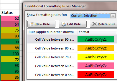
Now let’s say you wanted to color code based on ranges of values. For example, values of 90-100 would be green, 80-89 would be orange, 70-79 would be yellow, 60-69 would be pink, and everything else would be red.
The best way to accomplish this is to use Home, Conditional Formatting, Highlight Cells Rules, Between. That way, each rule is mutually exclusive. A value can’t fall between 60-69 and 70-79 at the same time.
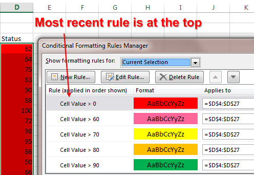
Another way to build the rules is to define a rule for values greater than 0 to be red. Then define a rule for values greater than or equal to 60 to be pink. Continue in order with each range, from smallest to largest. It’s crucial to go in this order because each new conditional formatting rule you create goes at the top of the list. If the last rule that you define is red for values greater than zero, it will appear at the top of the Conditional Formatting Rules Manager. And since every value is greater than zero, all of the values will be red. If you already have the rules in the wrong order, however, you can select a rule and use the up/down icons to reorder the rules in the list.
APPLYING COLORS QUICKLY
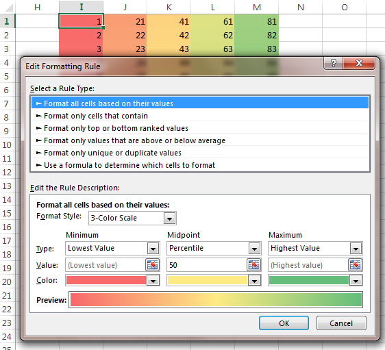
Excel 2007 introduced a new conditional formatting option called a Color Scale. This option eliminates the need to set up many rules. Choose a range of numbers and then select Home, Conditional Formatting, Color Scale. Choose one of the built-in three-color choices. Using a color scale, the numbers are assigned various shades of red, yellow, and green based on the number selected.

August 2016


