EXCEL: CREATING TERRITORIES

GROUP SELECTION

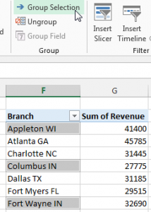
Let’s say that your data set includes a branch field indicating the city where the sale originated. You want to combine the branch office results into four regions. Prior to Excel 2013, you would have to use the Group Selection process. After creating a pivot table with Branch Office as the Row and Revenue as the Values, select each branch of the first territory. This involves clicking on the first branch and then holding down the CTRL button while you select all the other branches in that territory.

Figure 1

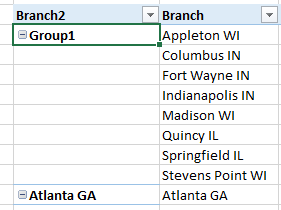
From the Options tab of the Excel 2010 ribbon (renamed to Analyze in Excel 2013), select Group Selection. This creates a new field called Branch2 with a territory name of Group1.

Figure 2

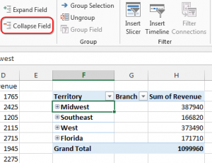
Visit the Design tab of the Ribbon and select Report Layout, Show in Tabular Form, and Repeat All Item Labels. Where the default Group1 name appears in the pivot table, type in the name of the territory.

Figure 3

Repeat these steps for each territory.

Figure 4

Even the Excel macro recorder won’t correctly record this process, so you’ll have to go through all the steps again the next time you need to create a pivot table with the same territories.

Figure 5

THE FASTER PROCESS

To make a region/territory table in Excel 2013, follow these steps:

Copy the branch column and paste it to a blank section of the worksheet. Make sure to leave at least one blank column between your original data set and the copied version.

Select the copied branch column.

On the Data tab, select Remove Duplicates.

Figure 6

Accept all of the defaults in the Remove Duplicates dialog and click OK. Excel will report the number of records that have been deleted and how many unique values are left.

To the right of the Branch column, add a new heading called Territory. Fill in the correct territory name for each branch.

Select one cell in the two-column Branch/Territory table. On the Home tab of the ribbon, select Format as Table and choose any of the Table Styles shown.

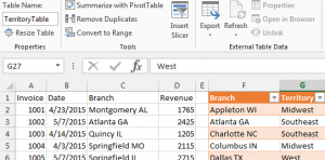
A new Table Tools Design tab will appear in the ribbon. On the right side of this tab, rename the table from Table1 to TerritoryTable.

Figure 7

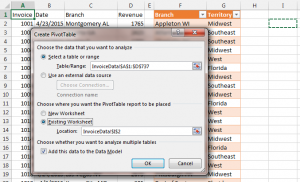
You now have two data sets. The original data set includes many detail rows. The smaller TerritoryTable contains just one entry per branch office. Select one cell in the original data set and choose Insert, Pivot Table. The Create Pivot Table dialog box contains a new checkbox in Excel 2013 called “Add This Data to the Data Model.” While not very descriptive, by checking the box, any fields from any table in your workbook can be included in the model.

Figure 8

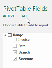
Build the pivot table by choosing Branch and Revenue in the Pivot Table Fields panel. Notice there’s an extra row below Pivot Table Fields offering “ACTIVE | ALL.” Click All to see fields from the TerritoryTable that can be added to the panel.

Figure 9

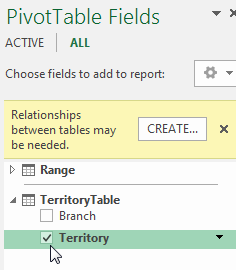
From the top of the Pivot Table Fields list, drag Territory to be the first field in the Rows area. A warning will appear that “Relationships Between Tables May Be Needed.”

Figure 10

Click the Create… button to open the Create Relationship dialog. There are four fields in the Create Relationship dialog. From the Table dropdown, choose Range to indicate the original Excel data set. In the Column (Foreign) dropdown, choose Branch. In the Related Table dropdown, choose TerritoryTable. In the Related Column (Primary) dropdown, choose Branch.

Figure 11

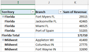
When you click OK, the pivot table will update to include the Territory column from the secondary table as well as the Branch and Revenue column from the original data set.

Figure 12

When you need to repeat these steps for additional pivot tables, simply copy the TerritoryTable to the new workbook and remember to check the box for “Add This Data to the Data Model” when creating the pivot table.

Selecting the checkbox for the Data Model actually loads the Power Pivot engine behind the scenes. Microsoft tried to convince enterprise customers to pay extra for Office Pro Plus so they could use Power Pivot. While the full add-in allows for loading millions of rows into Excel and a new DAX formula language, this nice feature of creating pivot tables from multiple tables is built into all versions of Excel 2013.