EXCEL: NONCONTIGUOUS SELECTIONS

ADD TO SELECTION

NO MOUSE NEEDED

Let’s say that you want to apply a Color Scale to the data cells in Figure 1. This means you need to select cells B4:D8, G5:I8, and D11:F13. Start by selecting cell B4. To select the first block of data, hold down Ctrl+Shift and press the down arrow (↓) and then the right arrow (→). This common keyboard trick selects all the way down to the bottom and the right edge of the data.  

Figure 1    

After selecting the first cell range, most people would switch to using the mouse. But it’s faster if you can keep your hands on the keyboard. Press Shift+F8. You’ll see the words “Add to Selection” in the status bar at the bottom of the Excel screen.  

Move the cell pointer to the next section of data: Ctrl+↓, Ctrl+→, Ctrl+↓, and then ↓. The original range, cells B4:D8, stays selected while you move the cell pointer outside of the range.  

To select the second range, hold down Ctrl+Shift and press ↓ then →. You’ve now selected B4:D8 and D11:F13 (see Figure 2). But now the “Add to Selection” is gone from the status bar. Press Shift+F8 to return to Add to Selection mode.  

Figure 2  

Move the cell pointer to cell G5. Hold down Ctrl+Shift and press ↓ then → to select the third block of cells (see Figure 3).  

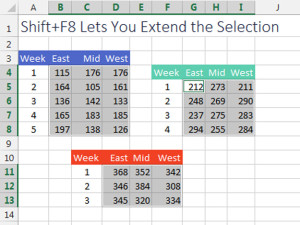
Figure 3  

EXTEND SELECTION

Many people haven’t seen Add to Selection. Instead, they have encountered the annoying Extend Selection mode. This usually happens when you try to press F9 to recalculate but accidently press F8 instead. In Extend Selection mode, any click of the mouse will select from the active cell to the newly clicked cell, obliterating any previous selection. While I’ve never found a good reason to use Extend Selection, there clearly are times when using Shift+F8 for Add to Selection will save time.  

GO TO SPECIAL

FAST SELECTION

Before using Add to Selection, you should consider if there’s a way to solve the problem using Go To Special. In Figure 1, the fact that the Weeks are stored as numbers (for example, cells A4:A8) preclude any useful way to utilize Go To Special.  

But if you adjust the spreadsheet to store the weeks as text, Go To Special becomes a fast and viable solution. Change cell A4 to “Wk 1” and drag down so the week number is always text (see Figure 4). Then follow these steps:  

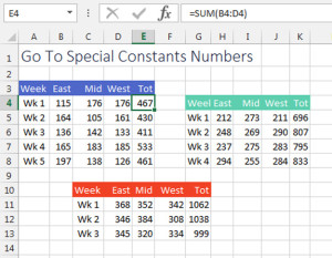
Figure 4    

1. Press Ctrl+A to select all the cells. The Go To Special dialog always takes a larger selection and makes the selection smaller.

2. On the Home tab, click on Find & Select, Go To Special.

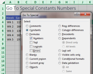
3. In the Go To Special dialog, choose Constants. This will make the four checkboxes for Numbers, Text, Logicals, and Errors become active.

4. Uncheck Text, Logicals, and ­Errors, leaving only Numbers checked (see Figure 5).

Figure 5  

5. Click OK.

The result is the same as using Shift+F8, but it takes less time. As an added benefit, Go To Special will exclude any formula cells that might exist in total columns or total rows. This is important when you are using any of the data visualization tools on the Conditional Formatting dropdown.  

COMPARE TWO COLUMNS

Here’s a little-known trick using Go To Special. Say that you have two columns of numbers that should be identical. You can identify the cells that have differences using Go To ­Special.  

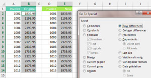
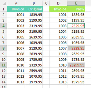
First select the column where you want to find the differences. Then add the original column to the selection. On the Home tab, select Find & Select, Go To Special, Row Differences (see Figure 6). When you click OK, only the items in the new column that are different from the original column will be selected. Apply a red font, and you can quickly mark all the cells that have changed (see Figure 7).  

Figure 6  

Figure 7    

SF SAYS

GREATER EFFICIENCY

Add to Selection and Go To Special are both very obscure and difficult to discover randomly. In the right situations, however, they can each save a lot of time.