Excel: TOP-LEVEL BUDGET VS. DETAIL-LEVEL ACTUALS

DATA MODEL

There was never an easy way to join the top-level budget numbers and the detail-level actuals.

You certainly couldn’t do a VLOOKUP from Actuals to Budget nor from Budget to Actuals. The new Excel 2013 Data Model finally allows you to join the Actuals data set and the Budget data set into a single pivot table.

The technique involves building a pivot table using the Excel 2013 “Data Model.” This generic-sounding term is designed to sound boring. While Microsoft wants you to invest in Office 2013 Pro Plus to unlock all of the features of Power Pivot, the fact is that a lot of the functionality is already in  the core Excel 2013 but disguised with the term “Data Model” instead of Power Pivot.

CREATE TABLES

Start with a single Excel workbook that has the Budget data on one sheet and the Actuals data on another sheet. Go to each tables and press Ctrl+T to declare them as official Tables. On the surface, this applies some nice formatting to the data. More importantly, it also makes the data sets eligible for the Data Model.

Before going further, you should visit the Table Tools tab in the ribbon and assign each table a meaningful name such as ActualsTable and BudgetTable instead of Table1 and Table2. This step isn’t necessary, but it’s a good best practice.

It’s likely that both tables have fields in common. For example, both might have region. Both might have product. It’s likely that both have date, although the invoice data likely includes daily dates while the budget data likely includes only the month-ending date. Your pivot table report usually has fields along the top (Column fields) and along the left side (Row fields). You are limited that in  you can only use the fields in common to both data sets as the Row and Column Fields in the pivot table.

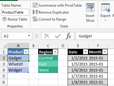
Here’s the critical step. For each field in common, you need to build a tiny table that lists all of the unique values in that field, such as the products or regions. This might be a one-column table with just a few records. Take the time to create this data, convert it to a table with Ctrl+T, and assign each a name, such as ProductTable. I’ll call these Joiner tables. When you create the pivot table, your row and column fields must come from the tiny Joiner table instead of from the Actuals or Budget table.

In the case of the mismatched dates, create a calendar table that includes all dates in either data set. Then add a reporting column that shows the month or quarter name.

THE PIVOT TABLE

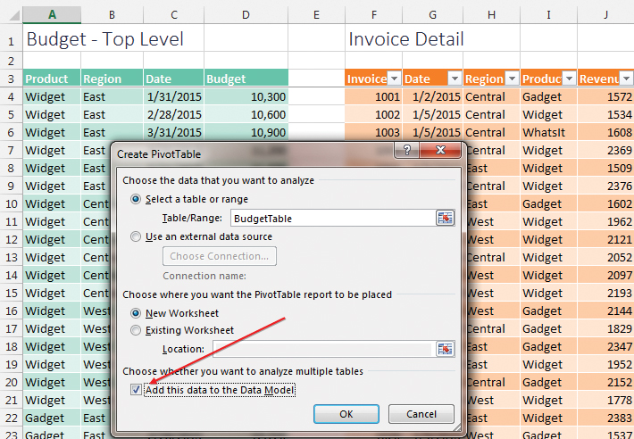
Select one cell in your Budget table. In Excel 2013, choose Insert, Pivot Table. Be sure to check “Add this data to the Data Model” at the bottom of the dialog box.

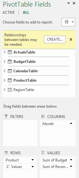
A blank pivot table is created. The PivotTable Fields list initially shows you only the records in the Budget table. But as we discussed last month, there’s a new setting in the  ­dialog offering ACTIVE | ALL. This is initially set to show only the active Budget table. Instead, click ALL, and you’ll see both the Budget and Actuals tables as well as each of the small Joiner tables.

As you build the pivot table, all of the numbers will initially appear wrong. This is normal. Build the pivot table to include:

* Sum of Budget from the Budget Table in the Values area.

* Sum of Revenue from the Actuals Table in the Values area.

* Month from the Calendar Table in the Columns area.

* Product from the Product table or Region from the Region table in the Rows area.

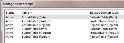
A large yellow warning box appears at the top of the Pivot Table Fields list saying that “Relationship Between Tables May Be Needed.” Click the Create button and define these relationships:

* BudgetTable Date to CalendarTable Date.

* ActualsTable Date to CalendarTable Date.

* BudgetTable Region to RegionTable Region.

* ActualsTable Region to RegionTable Region.

* ActualsTable Product to ProductTable Product.

* BudgetTable Product to ProductTable Product.

As soon as you define the sixth relationship, the yellow warning box goes away and the pivot table shows the correct numbers. As you can see, the Values field has been moved to the Row fields in order to compare Budget to Actuals.

The natural next step for this pivot table is to calculate Variance to Budget. This is where Microsoft gets you. In order to create calculated fields inside the pivot table, you need to upgrade to Pro Plus in order to get the full Power Pivot add-in.

SF SAYS

There are features for building more advanced pivot tables that are advertised as part of the Power Pivot add-in that comes with Office 2013 Pro Plus, but some are already available in the regular version of Excel 2013 under the guise of the Data Model.