Excel: Iterating a Function 359 Times

THE QUESTION

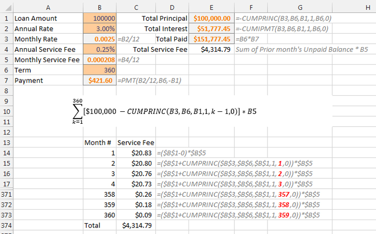
Each month, there’s a service fee calculated as 0.000208 times the unpaid balance from the prior month. Calculating the total service fee required 360 separate formulas. Figure 1 illustrates a sample calculation. The loan terms are entered into the orange cells in B1:B6. Formulas in the grey cells easily calculate the monthly payment, total principal, and total interest.

But how can you calculate the total service fee in cell E4? There’s a similar—but different—calculation happening each month. For example, in Month 7, you multiply the service fee rate by $100,000 (the cumulative principal paid through Month 6). Every month, you’re changing that formula to calculate the cumulative principal for the previous month.

CUMPRINC

While I frequently use PMT to calculate loan payments or PPMT and IPMT to build amortization tables, I had never really used CUMPRINC before. The function calculates the total principal paid on a loan from period x to period y. The syntax is =CUMPRINC(Rate, Term, Loan Amount, Start Month, End Month, Payment Type). To figure out the cumulative principal paid in the first 12 months, for example, use 1 as the start month and 12 as the end month (fourth and fifth arguments, respectively).

For those of you familiar with PMT, be aware that CUMPRINC can’t accept a negative loan amount. Thus, the result of CUMPRINC will always be negative.

For a 360-month loan, you need to calculate the cumulative principal for Months 0 through 359. In Figure 1, this is done with 360 rows of formulas, stretching to row 373. The formulas in cells D15:D373 illustrate how the fifth argument of the CUMPRINC function needs to increase from 1 to 2 to 3, and so on, up to 359. What if you had one formula where you specified that a particular argument should be run for all of the numbers from 0 to 359?

CUMPRINC can’t calculate the cumulative principal for Month 0 because the result would be 0. Therefore, in the rest of the calculations in this article, I will be iterating from 1 to 359 instead of from 0 to 359. So the goal is to find a single formula that can calculate CUMPRINC(B3,B6,B1,1,{1 to 359},0).

USE ROW

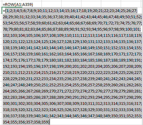
There’s a clever function called ROW that returns the row number of a cell. For example, =ROW(A17) is 17. This might not seem particularly useful, but you can send a range of cells to the ROW function. For example, =ROW(A21:A24) will return four values: {21,22,23,24}. In a similar fashion, =ROW(A1:A359) will return the numbers from 1 to 359. (See Figure 2.)

With =CUMPRINC(B3,B6,B1,1,ROW(A1:A359),0), Excel will actually do the calculation 359 times. You have to send those 359 answers into an accumulation function, such as SUM or AVERAGE. Otherwise, you will see only the result of using 1 as the fifth argument. So in this case, you would use =SUM(CUMPRINC(B3,B6,B1,1,ROW(A1:A359),0).

Since this is an array function, remember to press Ctrl+Shift+Enter after you enter the formula. The end result is a bit of a miracle—the one formula will replace 359 rows of formulas. Anytime that you need to repeat a function for sequential values from x to y, you could pull out the ROW() trick to insert many numbers where normally a single number would go.

To avoid the need for the keystroke combination, use SUMPRODUCT instead of SUM. This will help avoid any problems should people unfamiliar with array formulas edit the formula. SUMPRODUCT expects arrays, so there’s no need for the three-key combination.

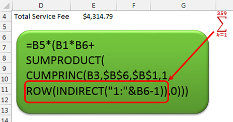
Inserting or deleting rows could change the argument in ROW(A1:A359). Hard-code that formula by using ROW(INDIRECT(“1:359”)). To make the formula flexible so you can change the term of the loan, incorporate that cell (B6) by using ROW(INDIRECT(“1:”&B6-1)).

FINISHING THE CALCULATION

For each of the 360 months, you’re subtracting the previous month’s CUMPRINC from the original loan amount and then multiplying that result by the monthly service fee in cell B5. From algebra, you might remember that 360 5 (a-b) is the same as (360 5 a)-(360 5 b).

The -(360 5 b) portion comes from the SUMPRODUCT formula that includes CUMPRINC and ROW. And it’s already negative because CUMPRINC returns a negative answer.

It might sound odd at first, but the (360 5 a) portion is the loan amount times the term: B1 5 B6. Thus, the final formula to calculate the total service fee is =B5 5 (B1 5 B6 +SUMPRODUCT(CUMPRINC(B3,$B$6,$B$1,1,ROW(INDIRECT(“1:”&B6-1)),0))). (See Figure 3.)

SF SAYS

This technique forcing Excel to repeat a function multiple times in a single cell can be applied to many other business calculations, such as extracting multiple matches in a lookup.