Excel: Visualizing Positive and Negative Changes

THREE TRIANGLES

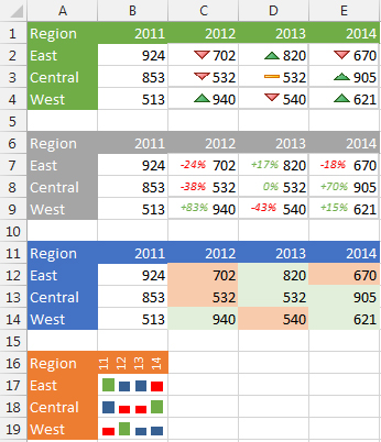
Microsoft added icon sets in Excel 2007, but the set they call Three Triangles debuted in Excel 2010. It’s essentially a green up indicator, a yellow flat indicator, and a red down indicator. You will use some helper  cells to make this work.

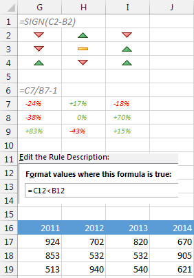
In Figure 2, the helper cells are shown in columns G through I, but you could also put them in columns AX through AZ or somewhere else outside of anyone’s view. Follow these steps to set up the icon set:

1. In cell G2, enter the formula =SIGN(C2-B2). This function shows all decreases as -1 and all increases as 1. In the rare case where a number is unchanged, the result is 0. Copy that formula to cells G2:I4.
2. Select G2:I4. Use Home, Conditional Formatting, Icon Sets, Three Triangles. The icons will appear on the left edge of the cell, and the result of the SIGN function appears on the right edge of the cell.
3. With G2:I4 selected, choose Home, Conditional Formatting, Manage Rules. Click Edit Rule.
4. In the bottom half of the Edit Formatting Rule dialog, choose Show Icon Only. (This setting isn’t available in Excel 2007.) Click OK once for each of the two dialog boxes that are open. The 1, 0, and -1 numbers are hidden, but the icon still appears on the left edge.
5. On the Home tab, choose the Center icon in the Alignment group to center the cell contents.
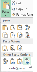
6. Copy cells G2:I4. Select cell C2. Open the Paste dropdown on the Home tab. Choose Linked Picture, the last icon in the dropdown list (see Figure 3).

It’s important that the width of the helper cells in columns G:I match the widths of columns B:D. Both sets of columns have to be wide enough to accommodate some space, the icon, and the number. To eliminate the need for extra width, skip Step 5.

CUSTOM NUMBER FORMAT

In Figures 1 and 2, rows 7-9 communicate the size of the increase or decrease. They also rely on helper cells and a linked picture. Follow these steps to get that result:

1. In cell G7, enter the formula =C7/B7-1. Copy that formula to cells G7:I9.
2. With cells G7:I9 selected, press Ctrl+1 to open the Format Cells dialog. On the Number tab, choose the Custom category and enter +0%;[Red]-0%;_+_00% into the Type box.
3. On the Home tab, choose a green, eight-point font, and align the text left. Click Increase Indent once.
4. Copy cells G7:I9. Select cell C2. Open the Paste dropdown and choose Linked Picture.

CONDITIONAL FORMATTING

Rows 12-14 use traditional conditional formatting that doesn’t require a helper cell. Follow these steps:

1. Select cells C12:E14.
2. Apply a light green fill to the selection by using the paint bucket icon on the Home tab.
3. Choose Home, Conditional Formatting, New Rule. In the New Formatting Rule dialog, click Use a Formula to Determine Which Cells to Format.
4. The formula has to be written to apply to the top-left corner of the selection. In Format Values Where This Formula Is True, type =C12<B12.
5. Click the Format button and the Fill tab, then choose a light-red color. Click OK in each of the three dialog boxes that are open. The cells with a decrease are highlighted in light red.
6. On the Home tab, choose the Fill Color dropdown and choose a light-green color. This color will show when the condition in Step 5 isn’t met, i.e., when there’s an increase or no change.

SPARKLINES

For rows 17-19, select the numbers in cells G17:J19. On the Insert tab, choose Column from the Sparkline group. Specify B17:B19 as the Location range. With the sparklines selected, use the Sparkline tab in the ribbon for these changes:

1. Open the Axis dropdown. For the Minimum value, choose Custom Value, 0, OK. In the same dropdown, set the Maximum to Same for All Sparklines.
2. In the Show group, select High Point and Low Point. Use the Marker Color dropdown to apply green and red to the high and low points, respectively.
3. The heading in B16 is created by typing in the values 11, 12, 13, and 14 and hitting Alt+Enter after each of the first three values. This will add a line break in the cell. To turn the text and alignment sideways, open the Format Cells dialog and go to the Alignment tab. Set the Text Orientation to 90 degrees. On the Font tab, select an eight-point font. Click OK.

Any of these techniques will show anyone at a glance which numbers are up or down from the previous year. Each takes just a few minutes to set up.