NESTED IF STATEMENTS
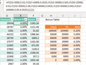
Consider the calculation for a bonus plan with multiple levels. With nested IF statements, you need to start at either the highest end or the lowest end of the bonus table. The formula in Figure 1, for example, starts at the low end of the table. The beginning of the formula (=IF(D2<5000,0.02,) means, “If this sale is less than $5,000, the bonus is 2%.” The final comma leads to the “else” portion of the IF function. The formula after the second comma is what happens once Excel decidesthe amount is greater than or equal to $5,000.
At this point, you add the next IF function to the formula:
=IF(D2<5000,0.02,IF(D2<10000,0.0225,.
For each additional level in the bonus table, you open a new IF function. When you get to the highest level, you don’t have to check for D2<250000. Once you know that the sale isn’t less than $100,000, you can assume it qualifies for the largest bonus: …IF(D2<100000,0.05,0.0525.
One of the most confusing parts of these formulas is counting the correct number of closing parentheses to use. You need one closing parenthesis for every IF statement. Here’s a helpful tip: Every version of Excel cycles through various colors for nested parentheses. The very first parenthesis is black. Excel then cycles through seven different colors of parentheses repeatedly, but it won’t use black again until you reach the final closing parenthesis. Keep typing parentheses until you type one that appears in the cell as black. Then you’ll know that you have a balanced number of closing and opening parentheses.
The final formula to create the bonus is 157 characters long and cumbersome to use: =IF(D2<5000,0.02,IF(D2<10000,0.0225,IF(D2<20000,0.025,IF(D2<25000,0.03,IF(D2<30000,0.04,IF(D2<40000,0.0425,IF(D2<50000,0.045, IF(D2<100000,0.05,0.0525)))))))).
APPROXIMATE MATCH VLOOKUP
Most VLOOKUP formulas end with a False argument, which tells Excel to find an exact match. When a VLOOKUP formula ends in True, Excel describes it as looking for an approximate match. A more accurate description is that Excel is trying to identify which range a value falls in—precisely what we need for the bonus calculation.
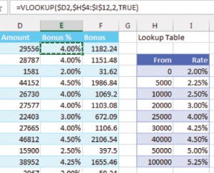
To use this version of VLOOKUP, your bonus table must start from the smallest amount and increase to the largest. Columns H:I in Figure 2 show how to convert the bonus table in Figure 1 to the lookup table used for finding ranges.
First, VLOOKUP will look for an exact match in the table. If you happen to have a sale for exactly $25,000, the VLOOKUP will return the value of 4%, just like a typical VLOOKUP would.
The powerful difference in the approximate match VLOOKUP occurs when the value isn’t found in the table. A regular VLOOKUP would return a #N/A error. The approximate match VLOOKUP will return the closest value in the table that’s less than the value you’re looking up.
For example, consider $29,556. When Excel can’t find this value in the table, it returns the 4% associated with the $25,000 row in the lookup table. It doesn’t matter that $29,556 is much closer to $30,000 than $25,000. Excel will always return the closet lower value. This makes it perfect for replacing a series of nested IF functions.
The formula in Figure 2 is only 31 characters: =VLOOKUP($D2,$H$4:$I$12,2,TRUE).
In a slightly bizarre twist of logic, Excel says that the fourth argument in a VLOOKUP formula defaults to TRUE if it’s left off, so you could shorten the formula to =VLOOKUP($D2,$H$4:$I$12,2). But I prefer to explicitly include the TRUE argument to remind me that it isn’t a typical VLOOKUP function.
While most lookup tables don’t have to be sorted, your table has to be sorted ascending when you use the approximate match VLOOKUP.
This version of VLOOKUP will still return the #N/A error if you try to find a value less than the first item in the table. For example, if a credit memo appears with an amount of -$5,600, the formula will return #N/A since this amount is less than the smallest item in the table. Depending on your rules for handling credit memos, the solution might be as simple as looking up ABS($D2) instead of $D2.

April 2015


