I remember receiving a telephone call in February 2002 from Jerry Kohl, who owned a chain of 20 women’s boutiques. He could get a report from the point-of-sale system showing all items sold in the last week across the entire chain. With 2,000 items for sale, no one was taking the time to glean anything useful from 40 pages of Excel data. Jerry knew how to use Excel to filter to all handbags and how to sort the report descending by quantity sold. But it was still a boring black-and-white printout.
Jerry had an awesome idea: Is there a way to filter to the top 10-selling handbags in the last week and display a one-page report with their images? Back then, I had to write some code in Visual Basic for Applications (VBA) to achieve the goal. But the report quickly became popular: It was hung up in the break room of all 20 stores, was posted on the bulletin board in the home office where the designers were working on new products for next season, and was posted near the buyers so each buyer knew to keep those 10 handbags in stock at each store.
When Microsoft released the new IMAGE function in late August 2022, I called Jerry to tell him that his idea was 20 years ahead of its time. That difficult dashboard of the top 10-selling products can now be done easily using one regular Excel formula.
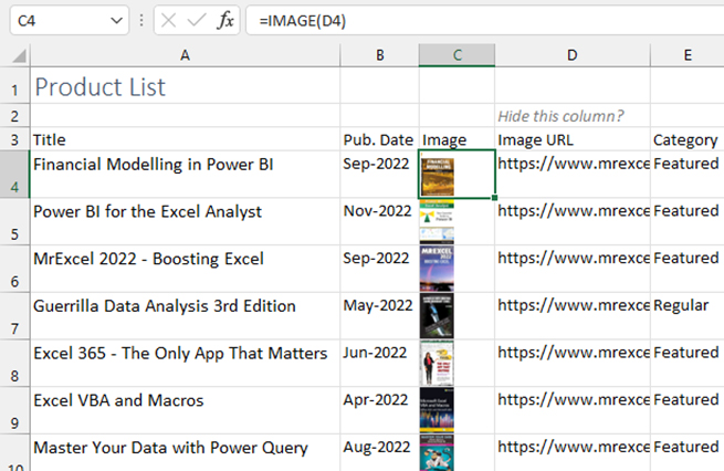
In the simplest form, the basic syntax is =IMAGE(“Image URL”). That’s all you need to display an image in a cell. When inserted among several rows of data, as shown in Figure 1, the images will be rather small. But hover over a displayed image in Excel, and a larger version of the image appears as a pop-up card next to the cell.

Optional arguments allow you to specify alternative text for the image and to control the sizing of the image within the cell.
EASY TO SORT OR FILTER
In the past, if you tried to insert an image into a cell, you had to be careful that the cell was never resized to be smaller than the image. In those cases, the images would fail to sort if they weren’t completely inside the cell. Filtering would work, but using the Advanced Filter to copy to a new range would cause the images to not appear in the output range.
The image returned by the new IMAGE formula is a new data type that resides in the cell. You can easily sort or filter the data, and the image moves with the cell that contains the formula. You can use Filter, Advanced Filter, and even the XLOOKUP, SORT, and FILTER functions to move the images to a dashboard or report.
EXCEL CACHES THE IMAGE
When you first display an image in the workbook, Excel will download the image, compress it to one-fifth the original size, and store the image in the workbook. If you copy the IMAGE formula to 100 rows of data, you’ll see each formula change to a #BUSY! error for a few seconds while the images are downloaded and processed. Once the images are stored in the workbook, it will be very fast to display the images, even if you’re using FILTER or XLOOKUP to deliver certain images to a dashboard.
While this strategy is generally good, I’ve heard of a few people who want to link to a dynamic image that changes throughout the day. This isn’t going to work with the IMAGE function. Once the image is cached in the workbook, Excel isn’t going to waste bandwidth pulling a new image at every recalculation of the workbook.
LARGER CELLS DISPLAY LARGER IMAGES
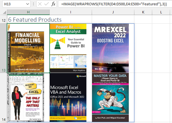
If you increase the height and width of the cell that contains the image, the image will resize proportionally until it matches the height or width of the cell. In Figure 2, rows 13 and 14 have a row height of 133. Columns H:J have a column width of 21. A single formula in H13 returns all six images shown in the figure: =IMAGE(WRAPROWS (FILTER(D4:D500,E4:E500="Featured"),3)).

Working from the inside of the formula, the FILTER function finds all the image URLs where column E indicates that the product is a featured product. Next, the WRAPROWS(…, 3) function wraps the list of matching image URLs into several rows of three columns each.
Finally, the IMAGE function retrieves the images of the six featured products. In this scenario, you wouldn’t need to show the hundreds of images in C4:C500. The FILTER function identifies the top products, and then the IMAGE function returns the image of just those items. That single formula in Figure 2 replaces more than 50 lines of VBA code that would have been required previously.


