Excel: Hack for Filtering a Pivot Table

COMPLEX FILTERS

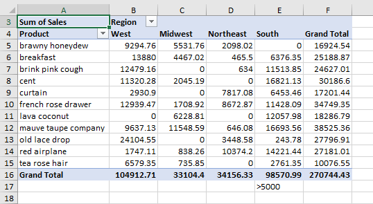
One area where this can present a challenge is applying a more complex filter to a pivot table. Consider the pivot table shown here.

Let’s say you wanted to only show rows where the total Sales for the South is greater than $5,000.

While there are plenty of ways to filter a pivot table, none solve the problem of filtering based on one column along the top of the pivot table. The drop-down menu in cell A4 offers a choice of Values Filters, Greater Than—but this will filter based on the Grand Total in column F.

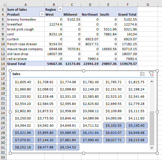
You could add a slicer based on the Sales column, but the slicer goes back to the original data set and filters rows. You don’t know which rows are ultimately going to add up to more than $5,000 in the South.

There is a hidden drop-down arrow that appears if you click the word “Sales” in the Pivot Table Fields pane. This drop-down lets you filter to Sales above or below a certain value, but, just like the slicer, this filters rows in the original data set.

The actual solution to the problem is found in a little-known button that you can add to the Quick Access Toolbar: the AutoFilter icon. Introduced all the way back in Excel 2003, the icon was never placed in the ribbon.

AUTOFILTER

To use this feature, you need to follow these steps once in order to make the features available:

1. Find the Undo button. It’s either located just above or below the ribbon in a strip known as the Quick Access Toolbar.
2. Right-click near the Undo button and choose Customize Quick Access Toolbar. The Excel Options dialog opens to the pane for Customize the Quick Access Toolbar.
3. A drop-down menu at the top-left of the dialog is set to Popular Commands. Change it to Commands Not In The Ribbon.
4. About 15 items down the left list box, you’ll see AutoFilter. Click on this command. In the center of the dialog, click the Add>> button to add the ­AutoFilter to the list box on the right.
5. Click OK to close the Excel Options dialog. You should now see the AutoFilter icon on the Quick Access Toolbar.

In general, when inside a pivot table, you aren’t allowed to use the Filter icon found on the Data tab of the ribbon. For example, if you selected E4 in Figure 1, you’d see that the Filter icon on the Data tab is grayed out.

Yet there is a hack available with the AutoFilter icon in the Quick Access Toolbar. Select the cell immediately below the South region total. In Figure 1, this is cell E17. Type a filter criterion in the cell, such as >5000. Examples of other criteria might be >0, 0, or <=10000. After pressing Enter, Excel will usually move to cell E18. Be sure to reselect the criteria cell in E17.

With cell E17 selected, click the AutoFilter icon in the Quick Access Toolbar. Several surprising things happen:

• Filter drop-downs will appear in cells B4:F4. (You would think this is impossible given that the Filter icon is grayed out when you select a cell in the pivot table.)
• Some parts of the Filter group are no longer grayed out, but they may not work as expected.
• The criteria cell in E17 is now hidden by the filter. If you want to change the criterion, you will first have to Clear the Filter (described below).

INCONSPICUOUS FUNCTIONALITY

Note that the AutoFilter isn’t part of the pivot table tools but is related to the Filter function on the Data tab. This means that some things won’t work the way you might expect. In particular:

• The Grand Total row will show the total of all rows—whether they’re visible or not. Changing the “Include Filtered Items in Totals” setting in the Subtotals drop-down on the Pivot Table Design tab won’t change the Grand Total.
• When you change the original data and click Refresh to update the pivot table, the AutoFilter criterion isn’t automatically reapplied.
• To clear the filter, open the drop-down menu in cell E4 and choose “Clear Filter from South.”
• To turn off the filter drop-downs, you need to select cell G4 and then toggle the Filter icon on the Data tab.

The scenario of filtering a pivot table based on the values for a particular column seem like it would be a frequent need. It’s unclear if Microsoft intended that the AutoFilter technique could be used in the fashion described here.

SF SAYS

Microsoft is working with a new pivot table interface in Excel Online to make it easier to find pivot settings.