EXACT MATCH
I’m a fan of VLOOKUP but concede that there are some things that make it difficult for people new to the function. The optional fourth argument in VLOOKUP specifies whether you want to find an approximate or exact match. The trouble is it defaults to the approximate match option. “Close” is never acceptable in accounting, so 99% of the VLOOKUP scenarios require the VLOOKUP to end with False or Zero. When a person new to Excel leaves off the fourth argument, some of the results will be correct and thus might lead the Excel rookie to think that the False isn’t needed. This is wrong and leads to incorrect results.
In contrast, XLOOKUP and XMATCH default to an exact match. If you don’t specify a match type in the optional fourth argument, you’ll automatically get an exact match. You can still do an approximate match if needed, such as if you’re calculating tax brackets or commission rates. But in 99% of the cases, you can leave the fourth argument out of XLOOKUP.
COLUMN INDEX NUMBER
The third argument in VLOOKUP is an integer that identifies the column number from which values should be returned. XLOOKUP replaces the integer with specific cell addresses. Say that you must do 12 columns of VLOOKUPs to return rates for January through December. Consider the formula =VLOOKUP($A2,RateTable,2,False). The 2 in the third argument says that you want to return the second column from the table. If that formula is in column B and you copy it to columns C, D, E, and so forth, Excel doesn’t know to increment the 2 to 3, 4, 5, and so on. Thus, you’re left with either editing the copied formula 11 times or applying some Excel trickery like using COLUMN(B:B) or a helper row to get the return column to move to the right.
With XLOOKUP, you specify cell addresses for lookup value, where to search, and what to return. For example, if your lookup table is in AA2:AM99, you might write =XLOOKUP($A2, $AA$2:$AA$99, AB$2:AB$99). Because of careful use of the dollar signs, the third argument will automatically move from AB$2:AB$99 to AC$2:AC$99 when you copy it to the right.

MORE IMPROVEMENTS
There are many other improvements brought about with XLOOKUP. Let’s take a look at some of the highlights.
Less-frequent calculations: Imagine an odd scenario where your lookup table starts in AA2 and extends 40 columns to the right. You need to get something from the 38th column using =VLOOKUP(A2,AA2:BN999,38,False). Although your VLOOKUP formula is really only looking at columns AA and BL, Excel will interpret the formula as having a dependency on anything from AA to BN. If anything inside the table changes, Excel’s intelligent recalculation engine will recalculate all of the VLOOKUP formulas. By only pointing to AA and BL, the XLOOKUP creates fewer formula dependencies with =XLOOKUP(A2,AA2:AA999,BL2:BL999).
Wildcard characters: If you used VLOOKUP to look up something that included the characters *, ?, or ~, there’s a good chance the formula didn’t work correctly. Those are wildcard characters, and VLOOKUP automatically treated them as wildcard characters. XLOOKUP turns off this behavior. If you truly want to do a wildcard lookup, then you can specify a 2 as the match type in the optional fifth argument.
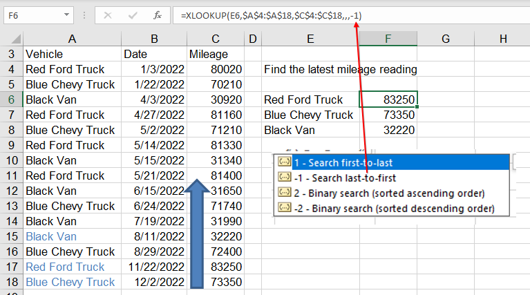
First or last match: VLOOKUP always returns the first matching value in the lookup column. Sometimes you might want to find the last match. For example, if you have a fleet of vehicles and record the odometer at each refueling, you can find the current mileage if you get the last match for each vehicle. By using the optional sixth argument, you can tell XLOOKUP to search from the bottom of the table.

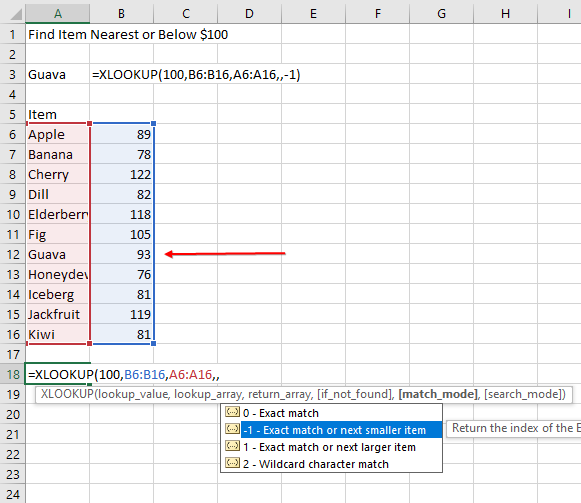
No sorting needed: It’s hard to believe, but with XLOOKUP you can search for the value equal to or next greater without the table being sorted. You would think this would take more time, but thanks to the new VLOOKUP algorithm introduced in 2018, the unsorted XLOOKUP calculation time is the same as a sorted VLOOKUP.

Replace 12 INDEX and MATCH with a single XLOOKUP: Some users love INDEX and MATCH. I’ve seen people use one MATCH and 12 INDEX formulas to solve the “return 12 months of VLOOKUP” problem. The amazing thing about XLOOKUP is that it supports dynamic arrays and will return all 12 months in a single formula.

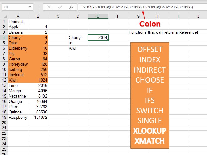
Return a value or a reference: A small handful of functions can return a value or a cell reference. For example, INDEX usually returns a value, but if you put the INDEX() next to a colon, Excel will instead return a cell reference. XLOOKUP and XMATCH have been written to return a cell reference. This will mostly be of use to formula tricksters, but it might allow you to add up all numbers associated with G/L account 2000 through 3500.

Whether you’ve been using VLOOKUP, HLOOKUP, or INDEX and MATCH, the new XLOOKUP offers improved functionality.
SF SAYS
XLOOKUP is shorter to write, faster to calculate, and less prone to errors than VLOOKUP.

October 2019


