CONDITIONAL FORMATTING
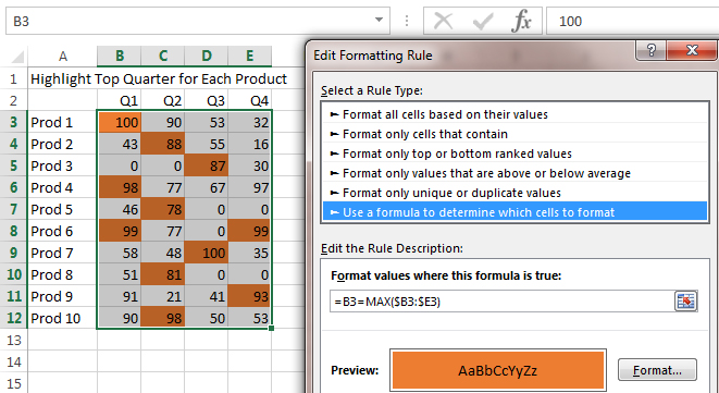
Cells B3:E12 of Figure 1 show the quarterly sales for several product lines. Use conditional formatting to call attention to the quarter in each row that had the largest sales compared to the other quarters. You need to build a formula for the top-left corner cell of the range. For cell B3, you want the cell to be highlighted when it’s equal to the largest value in B3:E3. In the conditional formatting rule, you could represent this as =B3=MAX($B3:$E3). Note that the reference inside the MAX function is a mix of relative and absolute references. The columns will always be B through E, but the row is allowed to change.

Once you have designed a formula that will work, add the conditional formatting for all the data:
- Select B3:E12.
- Select Home, Conditional Formatting, New Rule.
- In the New Formatting Rule dialog, choose “Use a formula to determine which cells to format.”
- Type =B3=MAX($B3:$E3) in the dialog box.
- Click the Format… button.
- In the Format Cells dialog, click the Fill tab and choose a fill color.
- Click OK to close the Format Cells dialog.
- Click OK to close the New Formatting Rule.
You should see the largest value in each row change color. In the case of row 8, where B8 and E8 are equal, both will be formatted.
REAL-LIFE COMPLICATIONS
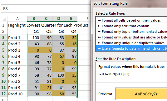
In a similar fashion, you can highlight the smallest value in each row by changing the formula in step 4 to =B3=MIN($B3:$E3). But after using this technique, you realize there are quarters where certain products aren’t offered for sale and the zero-quarter sales figures are getting highlighted (see Figure 2). Your manager wants you to ignore the zero values. Your goal is to highlight the smallest cell in each row that has a value greater than 0.
If you happen to be using Office 365 and have downloaded the February 2016 update to Excel, you could easily solve this using the new MINIFS function. The formula in step 4 would be =B3=MINIFS($B3:$E3,$B3:$E3, “>0”). But you’re likely to encounter many other users who don’t have the latest version of Excel, and the formula will stop working.
USE ARRAY FORMULAS
Although rarely used, the powerful array formula would allow you to test for the smallest value that isn’t zero, even in earlier versions of Excel. When used in a worksheet cell, array formulas require you to press Ctrl+Shift+Enter to complete the formula. But when used inside conditional formatting, they don’t.
You can start building this array formula from the inside. Consider the formula fragment IF($B3:$E3>0,$B3:$E3,“Ignore”). It says, “If B3:E3 is greater than zero, then use the number from B3:E3; otherwise, use a value of Ignore.” You could use any text in place of “Ignore”—even “” would work. In row 5, this formula fragment would produce the answers of Ignore, Ignore, 87, 30.
The MIN and MAX functions are designed to evaluate numbers in the range and to ignore any text values. If you ask for MIN(“Ignore”,”Ignore”,87,30), the answer will be 30. Thus, the next step in your formula is to take the MIN of the formula fragment: MIN(IF($B3:$E3>0,$B3:$E3,“”)).
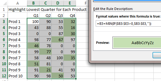
The final step is to see if the value returned by the MIN is equal to the value in B3. In the conditional formatting dialog, enter a test formula of =B3=MIN(IF($B3:$E3>0,$B3:$E3,“”)).
Because these array formulas are used so rarely, I didn’t expect the conditional formatting to evaluate an array formula. But if you follow the numbered steps and use this formula in step 4, it will correctly highlight the lowest value in each row while ignoring the zero values. In Figure 3, the array formula successfully highlights the 30 in row 5 instead of the zeroes in B5 and C5.

USEFUL TIPS
While editing the formula in the conditional formatting dialog, use care before pressing the left or right arrow key to move through the formula. By default, Excel will show an “Enter” status in the lower left of the Excel screen. As you press the left or right arrow key, Excel will insert cell references in the formula. To prevent this behavior, press F2 to toggle the Enter mode to Edit mode. You can now safely use the arrow keys to move through the formula.
SF SAYS
When used in worksheet cells, array formulas typically require pressing Ctrl+Shift+Enter to complete the formula.

June 2016


